3 Tutorial 3: Rule-based Approaches & Dictionaries
In Tutorial 3, you will learn….
- How to create a document-feature-matrix
- How to generate general descriptive statistics on your corpus
- How to use keywords-in-context
- How to conduct a dictionary analysis
For illustration, we’ll once again work with our data donations. By applying some of the preprocessing steps you just learned in Tutorial 2: Preprocessing, we prepare the search queries for analysis.
In short, we start building a pipeline for data preprocessing and data analysis (feel free to extend and improve this pipeline for your final analysis related to the term paper):
- We remove URL-related terms
- We remove encoding issues
- We transform texts to lowercase
#preprocessing pipeline
data <- data %>%

  #removing URL-related terms
  mutate(across("search_query",
                gsub,
                pattern = "https://www.youtube.com/results?search_query=",
                replacement = "",
                fixed = T)) %>%
  mutate(across("search_query",
                gsub,
                pattern = "+",
                replacement = " ",
                fixed = T)) %>%

  #removing encoding issues
  mutate(
         #Correct encoding for German "Umlaute"
         search_query = gsub("%C3%B6", "ö", search_query),
         search_query = gsub("%C3%A4", "ä", search_query),
         search_query = gsub("%C3%BC", "ü", search_query),
         search_query = gsub("%C3%9", "Ü", search_query),

         #Correct encoding for special signs
         search_query = gsub("%C3%9F", "ß", search_query),

         #Correct encoding for punctuation
         search_query = gsub("%0A", " ", search_query),
         search_query = gsub("%22", '"', search_query),
         search_query = gsub("%23", "#", search_query),
         search_query = gsub("%26", "&", search_query),
         search_query = gsub("%27|%E2%80%98|%E2%80%99|%E2%80%93|%C2%B4", "'", search_query),
         search_query = gsub("%2B", "+", search_query),
         search_query = gsub("%3D", "=", search_query),
         search_query = gsub("%3F", "?", search_query),
         search_query = gsub("%40", "@", search_query),

         #Correct encoding for letters from other languages
         search_query = gsub("%C3%A7", "ç", search_query),
         search_query = gsub("%C3%A9", "é", search_query),
         search_query = gsub("%C3%B1", "ñ", search_query),
         search_query = gsub("%C3%A5", "å", search_query),
         search_query = gsub("%C3%B8", "ø", search_query),
         search_query = gsub("%C3%BA", "ú", search_query),
         search_query = gsub("%C3%AE", "î", search_query)) %>%

  #transform to lower case
  mutate(search_query = char_tolower(search_query))
3.1 Document feature matrix
The “unit of analysis” in many automated content analyses are not whole texts, which computers cannot read or understand, but features.
As such, an additional part of our preprocessing/data analysis pipeline may be the transformation of texts to features:
Features can be individual words, word chains, entire sentences, numbers, or punctuation marks.
In automated content analysis, we often break down full texts to their features in a process called tokenization. This allows us to process texts automatically, that is, via the computer.
Take the first search query in our corpus, for example:
## [1] "barbara becker let's dance"- As a human, you would read this search query as a full sentence: The search query is focused on a person, “barbara becker” and a TV show “let’s dance”
- The computer, however, would break this query down to its single features1, here via the tokens() command, and interpret the output based on these. In short, it counts how often the letters “barbara”, “becker”, “let’s”, and “dance” occur.
## Tokens consisting of 1 document.
## text1 :
## [1] "barbara" "becker"  "let's"   "dance"
As such, the computer does not know that “barbara becker” is a person or that “let’s dance” is a TV show. This is of course important information to understand the search query and shows why automated content analysis has its pitfalls.
This approach of reducing content to relevant features, often via tokenization, is also called a “bag-of-words” approach. This means that content (i.e., a search query, a text) is interpreted solely based on the frequencies of distinct features. These features are assumed to characterize texts independent of their order or their context. So, “let’s” and “dance” are assumed to have the same meaning, independent of whether they occur closely together.
For this “bag-of-words” approach, we often work with a “document-feature-matrix”, here via the quanteda package:
A document-feature-matrix is a matrix in which:
- rows denote the documents that our corpus contains (here, our search queries)
- columns denote the features that occur across all documents
- cells indicate the frequency of a single feature in a single text
We create a DFM via the dfm() command to identify similarities or differences between feature occurrences across search queries and return the result via print():
## Document-feature matrix of: 6,032 documents, 8,945 features (99.97% sparse) and 0 docvars.
##        features
## docs    barbara becker let's dance one singular sensation mini disco superman
##   text1       1      1     1     1   0        0         0    0     0        0
##   text2       0      0     0     0   1        1         1    0     0        0
##   text3       0      0     0     0   0        0         0    1     1        0
##   text4       0      0     0     0   0        0         0    1     1        1
##   text5       0      0     0     0   0        0         0    0     0        0
##   text6       0      0     0     0   0        0         0    0     0        0
## [ reached max_ndoc ... 6,026 more documents, reached max_nfeat ... 8,935 more features ]
By inspecting the output, we learn that…
Our corpus consists of 6,032 documents, here single search queries. The first row of the DFM describes the first search query, the second the second search query, and so on.
We have 8,945 features occurring across all 6,032 documents. These features denote types, i.e., different features that occur in at least one search query. The first column of the DFM describes the first feature: the word “barbara”.
Cells describe how many times each feature occurs in each document. For example, the feature “barbara” occurs once in the first search query, but never in search queries 2-6. Other features, such as “mini” or “disco” occur in more than just the first search query.
In addition, our DFM is 99.97% “spare”. What does this mean? Sparsity can be understood as the number of cells that contain a 0: 99.97% of our cells contain a 0. This is not surprising - many words like “barbara” do likely occur in only few search queries and do not occur in most search queries.
3.2 Descriptive Statistics
3.2.1 Number of documents
First, you may want to know how many search queries our data contains. Using the ndoc() command, we see: about 6,000 queries (as already indicated by the DFM).
## [1] 60323.2.2 Number of features
Next, we may want to know how many features our corpus contains. Using the nfeat() command, we see: about 8,900 different features.
## [1] 89453.2.3 Feature Occurrence
Now, we may want to know how often each feature occurs:
- Using the featfreq() command, we extract the most common features
- Using the as.data.frame() command, we transform the object to a data frame.
- Using the rownames_to_column() from the tibble package, we then also save the name of each feature as a variable.
- Using the rename() command, we then rename the variable depicting the frequency of features as “occurrence”.
library(tibble)
features <- dfm %>%

  #calculate frequency of each feature
  featfreq() %>%

  #save result as data frame
  as.data.frame() %>%

  #save feature names (now as rownames) as variable
  rownames_to_column(., var = "feature") %>%

  #transform to tibble
  as_tibble() %>%

  #rename columns
  rename("occurrence" = ".")

#View result
head(features)
## # A tibble: 6 × 2
## feature occurrence
## <chr> <dbl>
## 1 barbara 2
## 2 becker 1
## 3 let's 11
## 4 dance 40
## 5 one 17
## 6 singular 1We for instance see that the word “dance” is relatively popular as it occurs around 40 times across all queries.
Using these commands, we can for instance see how often a specific feature - for example, the feature tagesthemen - is used in search queries:
## # A tibble: 1 × 2
##   feature     occurrence
##   <chr>            <dbl>
## 1 tagesthemen          1
Not often - only a single query uses the term!
3.2.4 Frequent & rare features
Next, we may want to know which features are most or least frequent.
We first display the 20 most frequent features…
##     the       %     der      of      in trailer     die deutsch     und     you     and      to     ist       a       i
##     241     124     117     113     107     106     102      93      90      82      77      76      71      70      61
##    song   vegan       2     ich  lyrics
##      53      53      52      52      50
… followed by the 10 least frequent features
##              becker            singular           sensation            superman                four            weddings
##                   1                   1                   1                   1                   1                   1
##             funeral                  45 wahlverwandschaften              goethe          beckenrand             sheriff
##                   1                   1                   1                   1                   1                   1
##               enjoy         tatsächlich         delfinrolle            germanys            topmodel            vorspann
##                   1                   1                   1                   1                   1                   1
##           handpumpe            together
##                   1                   1
3.2.5 Visualizing feature occurrences
A popular (but among many scientists now rather frowned upon) trend is to visualize frequent words with wordclouds.
Using the wordcloud() function, we visualize feature frequencies - the larger features displayed here, the more frequently they occur in our corpus.
To use the package, you need to install and activate the quanteda.textplots package.
Here, we visualize the most frequent 50 words:
library("quanteda.textplots")
textplot_wordcloud(dfm, max_words = 50, max_size = 10, color = "grey30")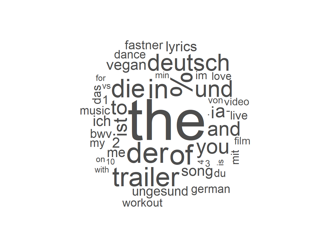
From the wordcloud, we can at least learn some things about our search queries - namely that they include different languages (German, English at the very least) and that news-related terms are not very frequent. Also, we could include some further preprocessing as the top terms for instance include punctuation or numbers which may not be too informative.
3.3 Keywords-in-Context
You need to be aware of the many (false) assumptions we rely on when using bag-of-words approaches. This includes the assumption that we can ignore the order and context of words to understand texts.
Oftentimes, doing so may be problematic: Suppose we think that the feature “interview” may be a good indicator for whether or not a person searches for news. After all, interviews are a common element in journalistic coverage; the feature “interview” may thus indicate news-related searches.
To analyze this, we may want to know which words are used in close distance to the feature interview (since this would be very indicative for how the term is used).
To answer this question, we can do a keywords-in-context analysis.
Keywords-in-context describes a method where we search for a certain keyword - for example interview - and retrieve words before or after this keyword.
Suppose we want to find any three features before and after the keyword interview to get a better sense of how the term is used.
The kwic() command gives us all n words before and after a pattern.
kwic <- data$search_query %>%
  tokens() %>%
  kwic(., pattern =  "interview", window = 3)

#Inspect results
head(kwic)
## Keyword-in-context with 6 matches.
## [text429, 2] mckinsey | interview |
## [text625, 2] chappelle | interview |
## [text1642, 2] mbappe | interview | laugh
## [text1766, 1] | interview | scholz
## [text1839, 5] longest ride cast | interview |
## [text1864, 3] jennifer lopez | interview |Here, we see that the feature “interview” is partly used to find news-related content - i.e., “interview scholz” - and partly used to find other types of content - i.e., “mckinsey interview”. So we should carefully consider whether (or not) to include the term when classifying news, for instance via dictionaries.
Later on, keywords-in-context may be helpful to create and enrichen our own dictionaries - for example, to find synonyms for “news” or “news story”.
3.4 Dictionary analysis
Let us now turn to a popular method related to automated content analysis: dictionary analysis.
Dictionaries are lists of features. Based on the manifest occurrence of certain features - for example, the words “news”, “tagesschau” and “intervuew” - the occurrence of a latent construct - for example, “news-related search” - is inferred.
Generally, we can distinguish between two types of dictionaries.
- Off-the-shelf dictionaries as existing word lists, often developed for other types of texts or topics. These are often used for sentiment analysis, for instance, and seen rather critical in the field of computational methods. We will therefore not discuss them here.
- Organic dictionaries as word lists you create manually for your type of text, topic, and the latent construct of interest.
We focus on these organic for further discussion see for example, Muddiman et al. (2019).
We may, for example, create an organic dictionary to classify search queries as news-related or not.
Imagine that you have already developed your own dictionary: a list of names of news outlets people may search for via Youtube. We could use the search of news outlets as a proxy for news-related searches.
You will find this list via Moodle under the folder “Data for R” (“whitelist_you.txt”).
As some outlets are included multiple times, we use the unique() command to only keep unique outlet names:
##           outlet
## 1          1LIVE
## 2        bayern1
## 3     br-klassik
## 4     BremenEins
## 5 bremenzwei9476
We now want to look up the occurrence of these outlets to draw inferences about the construct you are interested in (news-related search queries):2
Using this dictionary, we draw inferences about the occurrence of our latent construct of interest - news-related searches - by relying on the occurrence of outlet-related lusts we assume to describe the construct.
First, we transform our whitelist to a dictionary object, as is necessary within the quanteda framework:
Then, we look-up the occurrence of these words via three steps:
- We use the dfm_lookup() command to see which queries contain any of our outlet names.
- We use the convert() command to transform results to a data frame to check results.
- We use the cbind() command to merge the result with our data dataframe to have the classification and content-related variables in a single data frame.
- We use the rename() command to rename the variable with the name of our dictionary, “outlets.outlet”, to “classification_outlets” and, using the select() command, change the order of variables:
result_outlet <- dfm %>%

  #look up dictionary
  dfm_lookup(dictionary = dict_outlets) %>%

  #convert to data frame
  convert(., to = "data.frame") %>%

  #add to data dataframe
  select(outlets.outlet) %>%
  cbind(., data) %>%

  #rename
  rename("classification_outlets" = outlets.outlet) %>%

  #change order of variables
  select(external_submission_id, search_query, donation_platform, classification_outlets)
Let’s have a closer look at the results: Which search queries contain at least one outlet-name?
##   classification_outlets    n
## 1                      0 6007
## 2                      1   25
Overall, only 25 of our 6032 or 0.4% of search queries have been classified as news-related. Very few queries use search-related terms, at least based on the dictionary used here.
Next, we manually look at queries classified as “news-related searches” to get an idea of how well the classification worked:
##   external_submission_id                            search_query donation_platform classification_outlets
## 1                   4411            loriot das bild hängt schief           YouTube                      1
## 2                   5116 nytimes can we prevent another pandemic           YouTube                      1
## 3                   5628                               sonat vox           YouTube                      1
## 4                   5628                 sonat vox männerchor br           YouTube                      1
## 5                   5628        vox spain primer anuncio caballo           YouTube                      1
## 6                   6781             vice documentaries playlist           YouTube                      1
Results indicate some misclassification: For instance, the feature “bild” has been used as a proxy for the news outlet BILD - however, it may have another meaning in German (i.e., “picture”) and thus be misinterpreted here - which is why we should be validating results, something you will learn next.
3.5 Take Aways
Vocabulary:
- Tokenization is the process of breaking down articles to individual features, for instance words.
- Features are the result of such tokenization, often individual words in bag-of-word approaches.
- Document-feature-matrix is a matrix where rows identify the articles of your corpus and columns its features. Each cell indicates how often a feature occurs in a particular text.
- Dictionaries: Lists of words. Based on the manifest occurrence of these words, we draw conclusions about the occurrence of a latent construct, for example sentiment.
- Off-the-shelf dictionaries: Existing lists of features, often developed for other types of texts or topics.
- Organic dictionaries: Feature lists you created specifically for your type of text, topic, or construct of interest.
Commands:
- Counting documents & features: ndoc(), nfeat()
- Analyzing feature occurrences: featfreq(), topfeatures(), textplot_wordcloud(),
- Keywords-in-context: kwic()
- Transforming quanteda objects to other types of objects: convert()
- Dictionary analysis: dictionary()
3.6 More tutorials on this
You still have questions? The following tutorials & papers can help you with that:
3.7 Test your knowledge
You’ve worked through all the material of Tutorial 3? Let’s see it - the following tasks will test your knowledge.
3.7.1 Task 3.1
Writing the corresponding R code, add a second dictionary called dict_news that includes at least five synonyms for news-related terms (e.g., “news”)
Solution:
3.7.2 Task 3.2
Writing the corresponding R code, combine both dictionaries to identify news-related search queries.
Solution:
#look up
result_combined <- dfm %>%

  #look up dictionary
  dfm_lookup(dictionary = dict_outlets) %>%

  #convert to data frame
  convert(., to = "data.frame") %>%

  #add to data dataframe
  select(outlets.outlet) %>%
  cbind(., data) %>%

  #rename
  rename("classification_outlet" = outlets.outlet) %>%

  #add second dictionary
  cbind(dfm %>%

          #look up dictionary
          dfm_lookup(dictionary = dict_news) %>%

          #convert to data frame
          convert(., to = "data.frame") %>%

          #keep only classification variable
          select(news) %>%

          #rename
          rename("classification_news" = news)) %>%


  #change order of variables
  select(external_submission_id, search_query, donation_platform, classification_outlet, classification_news) %>%

  #create any dictionary match
  mutate(classification_combined = classification_outlet + classification_news)

#check results
result_combined %>%
  count(classification_combined)
## classification_combined n
## 1 0 5965
## 2 1 673.7.3 Task 3.3
Writing the corresponding R code, identify the external_submission_id of the person with the highest share of news-related searches.
Solution:
result_combined %>%

  #group by ID, here a single person
  group_by(external_submission_id, classification_combined) %>%

  #calculate share of news-related searches per oersin
  summarise(n = n()) %>%
  mutate(share = n / sum(n) * 100) %>%

  #only keep relative frequencies
  filter(classification_combined != 0) %>%

  #arrange by frequency
  arrange(desc(share)) %>%

  #get first rows
  head()
## `summarise()` has grouped output by 'external_submission_id'. You can override using the `.groups` argument.## # A tibble: 6 × 4
## # Groups: external_submission_id [6]
## external_submission_id classification_combined n share
## <int> <dbl> <int> <dbl>
## 1 7781 1 7 9.72
## 2 6781 1 8 8.16
## 3 7446 1 5 5.68
## 4 5628 1 4 4.26
## 5 10196 1 2 3.85
## 6 4172 1 3 3.063.7.4 Task 3.4
Writing the corresponding R code, calculate the mean percentage of news-related searches across people: On average, which percentage of Youtube searches are news-related?
(Spoiler: Based on your solutions, I saw that my question was not fully clear - which is why I added a simple solution here. We will get back to this later, in Tutorial 5)
Solution:
## [1] 1.110743Let’s keep going: Tutorial 4: Validating Automated Content Analysis
In this case, the default setting is set to the version 2 quanteda tokenizer which tokenizes text based on single words. It would, however, be possible to tokenize differently, for instance to break down content to the level of sentences or letters instead of words↩︎
This is, of course, not a good example for how to develop such a dictionary. In fact, developing a good organic dictionary takes a lot of time and resources, for instance by enriching it via keywords-in-context or theoretically deduced words - something you can then do for your seminar paper. Take the example as what it is: an example↩︎