Chapter 2 Getting Started with Data
2.1 R Packages
Packages are bundles of R functions. Some common R packages you will encounter:
ggplot2- has functions for plotting datadplyr- has functions for cleaning/manipulating datastats- has functions for statistical calculations and random number generation
The tidyverse is a set of eight common R packages used in data analysis. It includes ggplot2 and dplyr. When you start out in R, loading the tidyverse packages is a good idea.
2.1.1 Installing packages
To use a package for the first time, you need to install it. Do this in the console with the command install.packages(). E.g. to install the tidyverse packages:

Note the quotation marks around the package name.
2.1.2 Loading packages in an R session
Once a package is installed you needn’t install it again. But to access the package in a session, you must load it using library(). You will need to do this every time you enter a new R session.
library(tidyverse)If you run this code and get the error message “there is no package called ‘tidyverse’”, you need to first install it, then run library() again.
It is common practice to load packages at the beginning of your script file. E.g. in an R Markdown file, you should load the relevant packages in the setup chunk (the first code chunk):
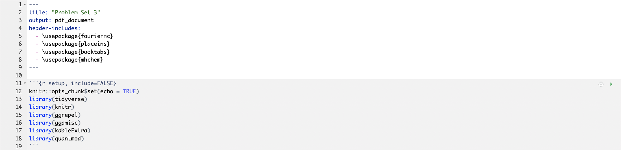
This will save you the hassle of remembering which packages you used and retyping them each time you enter a new session.
2.2 Loading Data
R has several inbuilt functions for loading data of various formats:
read.csv()for csv files (comma separated values)read.tsv()for tsv files (tab separated values)read.xlsx()for Excel files (from thereadxlpackage)read.dta13()for dat files (from thereadstata13package)read.table()for huge datasets
When loading data you must specify the exact file path in the argument (see below). If you don’t know how to find your file path, give it a google. Remember to name your dataset (i.e. assign your dataset to an R object)
The following code loads a csv file with data on the gender pay gap at various UK firms. Source: https://gender-pay-gap.service.gov.uk/. Locally the file is called ‘gender-paygap-2019.csv’ and it is assigned to the object name paygap:
paygap <- read.csv('./data/gender-paygap-2019.csv', header = TRUE)Note the extra argument, header = TRUE, which specifies that the first row of the dataset is a header. If your dataset has no header you should specify header = FALSE. Here the = operator is not used for variable assignment, but rather to specify an argument for the read.csv() function (this is the fundamental difference between the <- and = operators).
2.2.1 Viewing data
To view the entire dataset, use the View() command in the console. A table view of the dataset will open as a new tab. For large datasets it is not a good idea to use the View() command as it is very memory intensive.
Another way to see your data is to print the first or last few rows using the head() or tail() function. You can specify exactly how many rows as an additional argument (by default it will print six):
head(paygap, n = 5)## EmployerName DiffMeanHourlyPercent
## 1 A. & B. GLASS COMPANY LIMITED 19.0
## 2 Abbeyfield Wales Society 17.1
## 3 AMSRIC FOODS LIMITED 25.0
## 4 AMSRIC LIMITED 23.0
## 5 AMVALE MEDICAL TRANSPORT LIMITED 4.7
## DiffMedianHourlyPercent DiffMeanBonusPercent DiffMedianBonusPercent
## 1 4.0 42 45
## 2 28.2 NA NA
## 3 6.0 39 20
## 4 5.0 46 -47
## 5 3.9 NA NA
## MaleBonusPercent FemaleBonusPercent PropMaleTopQuartile
## 1 70 41 0.900
## 2 0 0 0.089
## 3 23 25 0.680
## 4 39 47 0.400
## 5 0 0 0.729
## PropFemaleTopQuartile EmployerSize
## 1 0.100 250-499
## 2 0.911 0-249
## 3 0.320 1000-4999
## 4 0.600 250-499
## 5 0.271 250-499To check the column names of your dataset, use colnames():
colnames(paygap)## [1] "EmployerName" "DiffMeanHourlyPercent"
## [3] "DiffMedianHourlyPercent" "DiffMeanBonusPercent"
## [5] "DiffMedianBonusPercent" "MaleBonusPercent"
## [7] "FemaleBonusPercent" "PropMaleTopQuartile"
## [9] "PropFemaleTopQuartile" "EmployerSize"To check the dimensions of your dataset (number of rows and columns), use dim():
dim(paygap)## [1] 153 10
2.3 Basic Data Structures
A variable refers to something that is measured. In the pay gap data each column contains data pertaining to a specific variable (employer name, employer size, etc). Data can be continuous, discrete, or categorical.
Continuous data can take an infinitely many values (real numbers).
Discrete data can take on countable values only (integer numbers).
Categorical data fall into a finite number of categories or distinct groups.
2.3.1 Data types in R
Every object in R has a data type. Below are the five elementary data types in R:
- character – e.g.
'abcd' - integer – integer numbers, e.g.
'2' - numeric – decimal numbers, e.g.
'2.21' - complex – complex numbers, e.g.
'2+2i' - logical – either
TRUEorFALSE
Objects may be combined to form larger data structures. Some common ones:
- vector – a one-dimensional array; there are two kinds of vectors:
- atomic vector – holds data of a single data type
- list – holds data of multiple data types
- matrix – a two-dimensional array; all columns have the same data type
- data frame – a two-dimensional array; columns may have different data types
You can check an object’s data type using class():
class(paygap)## [1] "data.frame"The data frame is indeed a common structure for tabular data. To check the data type(s) in the column DiffMeanHourlyPercent:
class(paygap$DiffMeanHourlyPercent)## [1] "numeric"Note the extract operator, $, which is used to extract a named element from an object (in this case extract a column from a data frame).