Chapter 5 Basic Data Modeling

5.1 Learning From Data

When two (or more) variables are related, you can build a statistical model that identifies the mathematical relationship between them. Data modeling has two important purposes:

prediction–predicting an outcome variable based on a set of predictor variables
causal inference–determining the causal relationships between variables

Using models to learn from data is an important part of statistics, machine learning, and artificial intelligence. Some examples of learning problems:

predicting the price of a stock 6 months from now, using economic data and measures of company performance
predicting which candidate will win an election, based on poll data and demographic indicators
identifying the variables causing global temperature and sea level changes
- https://climate.nasa.gov/evidence/
identifying patterns in images to train machine-learning algorithms
- https://qz.com/495614/computers-can-now-paint-like-van-gogh-and-picasso/

There are many approaches to building models to learn from data. Linear regression is one of the simplest. Although it predates the computer era, and more modern techniques have since been devised–such as neural networks, tree-based models, and ML–linear regression is still an important part of statistics and data science.

5.2 Simple Linear Regression

Linear regression is a technique for modeling linear relationships between variables¹.

In its simplest form, a linear model has one response variable and one predictor variable. The response should have some form of linear dependency on the predictor².

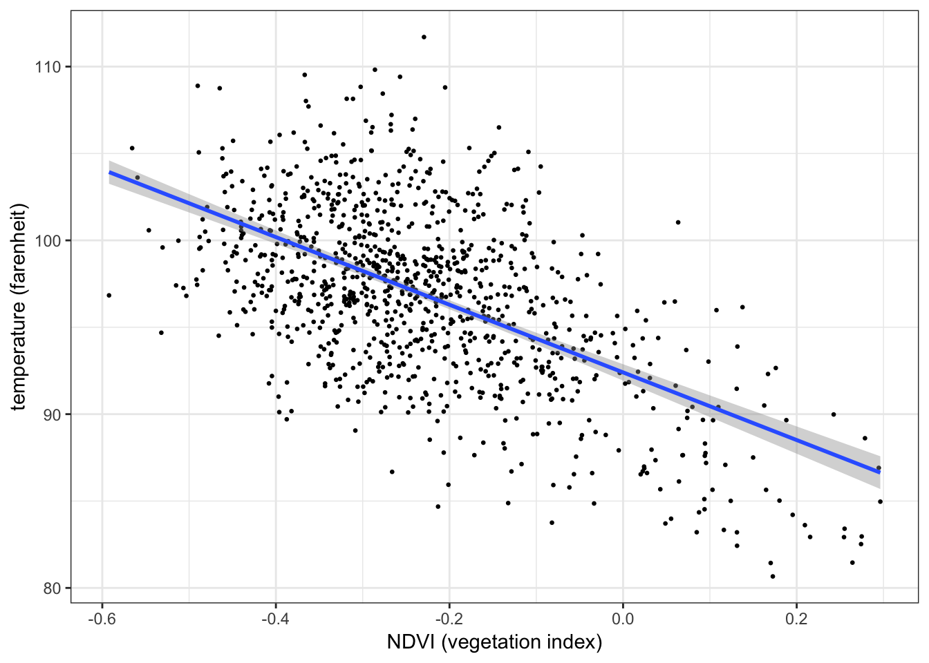
In linear regression, the relationship between the predictor and response is modeled using a linear function (a straight line). This is known as a regression line–you can think of it as essentially a line of best fit for the data.

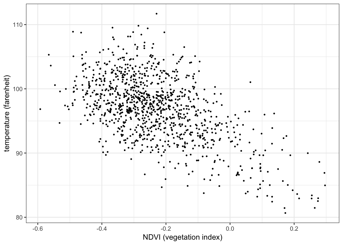
The plot below shows the relationship between temperature (response) and vegetation (predictor) from the NYC heatwave data, with a regression line overlaid³:

ggplot(aes(x = ndvi, y = temperature), data = nycheat) +
  geom_point(size=0.5) +
  stat_smooth(method='lm') +           # overlay regression line
  xlab('NDVI (vegetation index)') + ylab('temperature (farenheit)') +
  theme_bw()

5.2.1 Functional form

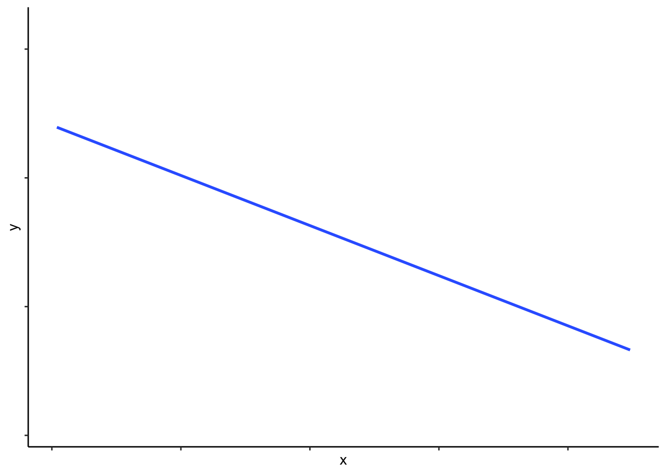
Figure 5.1: A simple linear function, of form \(y=mx+c\).

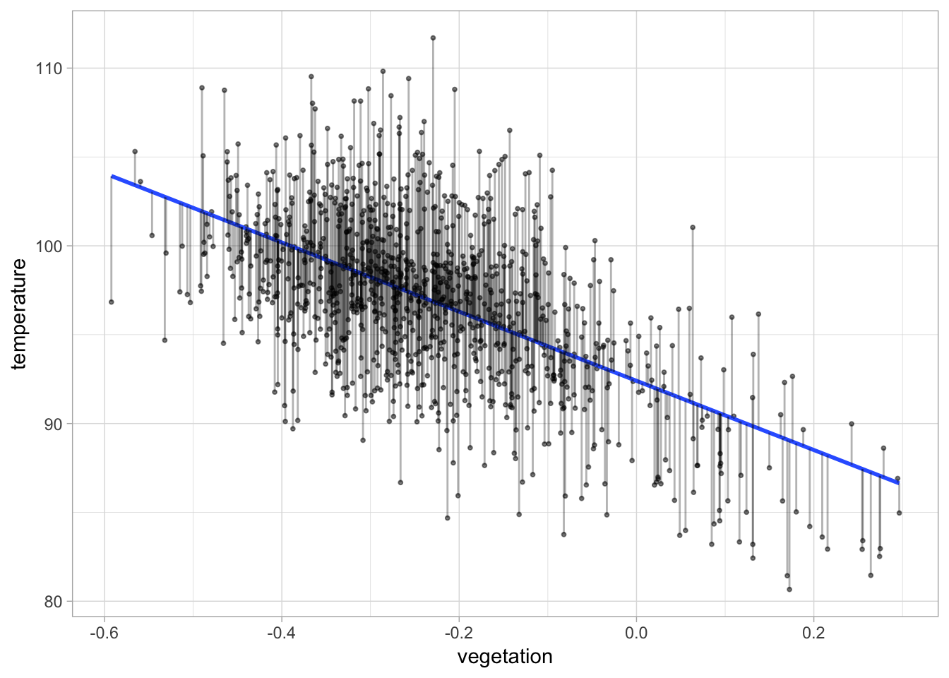
Figure 5.2: A linear function used to model the observed relationship between two variables (with error bars shown).

Any linear function is uniquely parametrized by two quantities–slope and intercept. You may be familiar with the equation for a straight line, \(y=mx+c\), where \(m\) is the slope and \(c\) is the \(y\)-intercept. When you assign values to the parameters \(m\) and \(c\), you can draw a straight line.

In linear regression there is a slightly different notational convention for describing the relationship between \(y\) and \(x\):

\[y_i = \beta_0 + \beta_1 x_i + \varepsilon_i\]

where:

\(y\) is the response variable
\(x\) is the predictor variable
\(\beta_0\) is the \(y\)-intercept of the regression line (the value of \(x\) when \(y=0\))
\(\beta_1\) is the slope of the regression line (the change in \(y\) for every unit change in \(x\))
\(\varepsilon\) is the error term, or the distance between each data point and the regression line
\(i\) denotes an individual observation in the data, where \(i = 1,...,n\) and \(n\) is the number of observations in the dataset

The main difference between this form and \(y=mx+c\) is the presence of an error term, \(\varepsilon\), in the equation. This is included because data points don’t fall exactly on the regression line. You can visualize the error term as the distance between the data points and the regression line–see the figure on the right.

The subscript \(i\) denotes an individual observation in the data. Its presence in the equation is essentially for describing the exact position of each data point in the plot. E.g. the 5th observation of \(y\) in the data is: \(y_{i=5} = \beta_0 + \beta_1 x_{i=5} + \varepsilon_{i=5}\).

You can also express the regression equation in matrix array notation, which omits the \(i\) subscript:

\[\boldsymbol{y} = \beta_0 + \beta_1 \boldsymbol{x} + \boldsymbol{\varepsilon}\]

where \(\boldsymbol{y}\) is a \(n \times 1\) matrix of the \(y\)-observations, \(\boldsymbol{x}\) is a \(n \times 1\) matrix of the \(x\)-observations, and \(\boldsymbol{\varepsilon}\) is a \(n \times 1\) matrix of the error terms, i.e.

\[ \begin{alignat*}{2} \boldsymbol{y} \hspace{0.5cm} &= \hspace{0.5cm}\beta_0 \hspace{0.3cm} + \hspace{0.3cm} \beta_1 \cdot \hspace{0.4cm} \boldsymbol{x} &&+ \hspace{0.5cm} \boldsymbol{\varepsilon} \\ \\ \begin{bmatrix} y_1 \\ y_2 \\ \vdots \\ y_n \end{bmatrix} &= \hspace{0.5cm} \beta_0 \hspace{0.3cm} + \hspace{0.3cm} \beta_1 \cdot \begin{bmatrix} x_1 \\ x_2 \\ \vdots \\ x_n \end{bmatrix} &&+ \begin{bmatrix} \varepsilon_1 \\ \varepsilon_2 \\ \vdots \\ \varepsilon_n \end{bmatrix} \end{alignat*} \]

5.2.2 The regression coefficients

The intercept and slope, \(\beta_0\) and \(\beta_1\), are known as the coefficients or parameters of a linear model.

The goal of linear regression (indeed any parametric modeling technique) is to estimate the parameters of the model.

In R, you can use lm() to perform linear regression and compute the coefficients. The required arguments are formula⁴ and data.

E.g. the following code regresses temperature on vegetation from the NYC heatwave data:

reg1 <- lm(formula = temperature ~ ndvi, data = nycheat)

You can view the results by calling summary() on the saved regression data:

summary(reg1)

## 
## Call:
## lm(formula = temperature ~ ndvi, data = nycheat)
## 
## Residuals:
##      Min       1Q   Median       3Q      Max 
## -11.8701  -2.8714  -0.0032   2.6661  14.8327 
## 
## Coefficients:
##             Estimate Std. Error t value Pr(>|t|)    
## (Intercept)  92.4019     0.2401  384.81   <2e-16 ***
## ndvi        -19.4644     0.8779  -22.17   <2e-16 ***
## ---
## Signif. codes:  0 '***' 0.001 '**' 0.01 '*' 0.05 '.' 0.1 ' ' 1
## 
## Residual standard error: 4.125 on 1019 degrees of freedom
## Multiple R-squared:  0.3254, Adjusted R-squared:  0.3248 
## F-statistic: 491.6 on 1 and 1019 DF,  p-value: < 2.2e-16

The coefficients are printed under Estimate. In this case the \(y\)-intercept of the model is estimated to be \(\beta_0 =\) 92.402 and the slope to be \(\beta_1 =\) -19.464.

Substituting these values into the regression formula gives the following equation:

\[\Longrightarrow \hspace{0.5cm} y_i = 92.40 -19.46 \; x_i + \varepsilon_i\]

This equation suggests that when vegetation index increases by 1, temperature decreases by 19.46\(^o F\).

5.2.3 Prediction from linear models

Once you have computed the regression coefficients, you have a linear model. You can now use this model to predict the value of the response variable for a given value of the predictor.

The predicted values of a linear model are points that lie on the regression line. A predicted value is typically denoted \({\skew{3}\hat{y}}\), where:

\[{\skew{3}\hat{y}} = \beta_0 + \beta_1 x\]

In the above example the predicted equation is \({\skew{3}\hat{y}} = 92.40 - 19.46 \; x\). This model predicts that if the vegetation index of an area is 0.2, its temperature will be \(92.40 - 19.46 \cdot 0.2 = 88.51 \; ^o F\).

Note that if \({\skew{3}\hat{y}} = \beta_0 + \beta_1 x\), this implies⁵ that:

\[y = {\skew{3}\hat{y}} + \varepsilon\]

i.e. the observed \(y\)-value (as seen in the data) is equal to the predicted \(y\)-value plus an error. Rearranging, you can also see that:

\[\varepsilon = y - {\skew{3}\hat{y}}\]

i.e. the error term is simply the observed \(y\)-value minus the predicted \(y\)-value.

In R you can use predict() to generate a vector of predicted values of a model⁶. In the argument you should specify the model you are using for prediction.

The following code generates a set of predicted values of temperature using the model specified above (reg1). The predicted values are assigned to a new variable in the data, temperature_prediction:

nycheat <- nycheat %>%
  mutate(temperature_prediction = predict(reg1))

If you were to plot the predicted response (\({\skew{3}\hat{y}}\)) on the predictor (\(x\)), you would find the data points lie on the regression line:

ggplot(data = nycheat, mapping = aes(x = ndvi, y = temperature_prediction)) +
  geom_point(size=0.5) +
  theme_minimal()

5.2.4 Extrapolation and its risks

Extrapolation refers to using models for prediction outside the range of data used to build the model.

E.g. in the heatwave data, values of vegetation index range from -0.6 to 0.25.⁷ If you tried to use the model specified above to predict temperature when vegetation index is 0.5, you would be extrapolating since there is no data to support your prediction for values in that range.

In general, extrapolation is risky because the linearity of a relationship is not guaranteed outside the range of observed data. In the heatwave data you can’t intuit how the relationship between temperature and vegetation evolves for higher or lower values of vegetation index. Theoretically it could look like this:

insert plot with nonlinear extension

If indeed the relationship is nonlinear outside the range of observed data, the linear model will yield invalid predictions of the response variable.

5.3 Multiple Regression

The linear model demonstrated above is known as a simple linear model since only one predictor variable is used to model the behavior of the response variable. In reality a response variable can be influenced by a number of factors–not just one–and thus it is often necessary to build a model with many predictors.

Multiple regression is a generalization of the simple linear model to include more than one predictor variable.

E.g. below is a correlation matrix of the numerical variables in the NYC heatwave data:

	temperature	ndvi	albedo	building_height	pop_density
temperature	1.0000000	-0.5704794	-0.6089282	0.3129929	0.0936772
ndvi	-0.5704794	1.0000000	0.3436937	-0.3301132	-0.0000113
albedo	-0.6089282	0.3436937	1.0000000	-0.1797287	-0.1074622
building_height	0.3129929	-0.3301132	-0.1797287	1.0000000	-0.0467194
pop_density	0.0936772	-0.0000113	-0.1074622	-0.0467194	1.0000000

Clearly temperature is correlated not only with vegetation, but also with albedo, building height, and (to a lesser extent) population density. In the following multiple regression model, all four variables are used as predictors of temperature:

reg2 <- lm(formula = temperature ~ ndvi + albedo + building_height + pop_density, data = nycheat)
summary(reg2)

## 
## Call:
## lm(formula = temperature ~ ndvi + albedo + building_height + 
##     pop_density, data = nycheat)
## 
## Residuals:
##      Min       1Q   Median       3Q      Max 
## -12.6189  -2.1516   0.1683   2.0384  13.5973 
## 
## Coefficients:
##                   Estimate Std. Error t value Pr(>|t|)    
## (Intercept)      9.563e+01  5.453e-01 175.379  < 2e-16 ***
## ndvi            -1.292e+01  8.159e-01 -15.831  < 2e-16 ***
## albedo          -3.667e-01  1.866e-02 -19.646  < 2e-16 ***
## building_height  1.685e-01  3.542e-02   4.758 2.24e-06 ***
## pop_density      2.283e-05  9.895e-06   2.307   0.0212 *  
## ---
## Signif. codes:  0 '***' 0.001 '**' 0.01 '*' 0.05 '.' 0.1 ' ' 1
## 
## Residual standard error: 3.444 on 1016 degrees of freedom
## Multiple R-squared:  0.5311, Adjusted R-squared:  0.5292 
## F-statistic: 287.7 on 4 and 1016 DF,  p-value: < 2.2e-16

As you can see each predictor has its own coefficient. The coefficient on any one predictor describes the change in the response for every unit change in that predictor, while holding the other predictors constant. This is important. In a simple (bivariate) linear model, the coefficient describes the change in the response for every unit change in the predictor. But in a multivariate linear model, the coefficient on a predictor describes its effect on the response, while effectively controlling for the other predictors. This is why the coefficient on vegetation in the multiple model is smaller than that in the simple model (-12.92 vs -19.64). The observed effect of vegetation on temperature is smaller when controlling for other variables.

Mathematically, a multiple regression model has the following functional form:

\[y_i = \beta_0 + \beta_1 x_{i1} + \beta_2 x_{i2} + ... + \beta_k x_{ik} + \varepsilon_i\]

where \(x_1, x_2, ..., x_k\) are a set of \(k\) predictor variables and \(\beta_1, \beta_2, ..., \beta_k\) are their coefficients. In this notation \(x_{ij}\) denotes the \(i\)-th observation in the \(j\)-th predictor variable.

In matrix notation:

\[\boldsymbol{y} = \boldsymbol{x} \boldsymbol{\beta} + \boldsymbol{\varepsilon}\]

i.e.

\[ \begin{bmatrix} y_1 \\ y_2 \\ \vdots \\ y_n \end{bmatrix} = \begin{bmatrix} 1 & x_{11} & ... & x_{1k} \\ 1 & x_{21} & ... & x_{2k} \\ \vdots & \vdots & \ddots & \vdots \\ 1 & x_{n1} & ... & x_{nk} \end{bmatrix} \cdot \begin{bmatrix} \beta_0 \\ \beta_1 \\ \vdots \\ \beta_k \end{bmatrix} + \begin{bmatrix} \varepsilon_{1} \\ \varepsilon_{2} \\ \vdots \\ \varepsilon_{n} \end{bmatrix} \]

5.4 Categorical Predictors in Linear Models

The examples thus far have demonstrated models with continuous predictor variables. You can in fact also include categorical variables as predictors in linear models.

E.g. in the heatwave data, the variable area is categorical with 6 levels/categories:

unique(nycheat$area)

## [1] crown heights brooklyn fordham bronx          lower manhattan east  
## [4] maspeth queens         mid-manhattan west     ocean parkway brooklyn
## 6 Levels: crown heights brooklyn fordham bronx ... ocean parkway brooklyn

Now consider the following multiple regression model, which regresses temperature on vegetation (continuous), albedo (continuous), and area (categorical):

reg3 <- lm(formula = temperature ~ ndvi + albedo + area, data = nycheat)
summary(reg3)

## 
## Call:
## lm(formula = temperature ~ ndvi + albedo + area, data = nycheat)
## 
## Residuals:
##      Min       1Q   Median       3Q      Max 
## -11.9071  -2.0304   0.0669   2.0477  12.6965 
## 
## Coefficients:
##                             Estimate Std. Error t value Pr(>|t|)    
## (Intercept)                 98.14913    0.34377 285.505  < 2e-16 ***
## ndvi                       -15.92828    0.79434 -20.052  < 2e-16 ***
## albedo                      -0.33964    0.01789 -18.988  < 2e-16 ***
## areafordham bronx           -2.26691    0.32416  -6.993 4.88e-12 ***
## arealower manhattan east    -3.44966    0.39219  -8.796  < 2e-16 ***
## areamaspeth queens          -1.68849    0.30736  -5.493 4.98e-08 ***
## areamid-manhattan west      -4.38913    0.42500 -10.327  < 2e-16 ***
## areaocean parkway brooklyn  -0.45976    0.37786  -1.217    0.224    
## ---
## Signif. codes:  0 '***' 0.001 '**' 0.01 '*' 0.05 '.' 0.1 ' ' 1
## 
## Residual standard error: 3.24 on 1013 degrees of freedom
## Multiple R-squared:  0.5863, Adjusted R-squared:  0.5834 
## F-statistic: 205.1 on 7 and 1013 DF,  p-value: < 2.2e-16

Note how each category appears as a separate predictor, with its own coefficient. Each category should be interpreted a dummy variable⁸.

Note also how one of the categories–Crown Heights Brooklyn–is missing. This is because R uses one of the categories as a baseline which the other coefficients are relative to. The baseline category is omitted from the output.

Recall the observed linear relationship between temperature and vegetation from the NYC heatwave data:↩
i.e. changes in the predictor variable should be associated/correlated with linear changes in the response variable. You can check the linear correlation of two variables by making a scatterplot or computing Pearson’s correlation coefficient. In the above example \(r=-0.57\).↩
You can overlay a regression line on a scatterplot by specifying + stat_smooth(method='lm'). The grey region around the line is its standard error. You can remove this by specifying se = FALSE as an additional argument.↩
The regression formula, specifying the response and predictor variables, in the form y ~ x.↩
Using the fact that \(y = \beta_0 + \beta_1 x + \varepsilon\).↩
Specifically, it generates a set of predicted values for each observation of the predictor variable.↩
For reference ^↩
A dummy variable can only take two values, 0 and 1. E.g. \[\texttt{areafordham bronx} = \cases{1 \;\;\; \text{if area} = \text{fordham} \\ 0 \;\;\; \text{if area} \neq \text{fordham}}\] Thus when predicting temperatures in Fordham, the equation is: \[\text{temp}_{fordham} = 98.15 - 15.93\text{*veg} - 0.34\text{*albedo} - 2.27\] When predicting temperatures in Maspeth: \[\text{temp}_{maspeth} = 98.15 - 15.93\text{*veg} - 0.34\text{*albedo} - 1.69\]↩