Chapter 5 XGBoost

XGBoost is a set of open source functions and steps, referred to as a library, that use supervised ML where analysts specify an outcome to be estimated/ predicted. The XGBoost library uses multiple decision trees to predict an outcome.

The ML system is trained using batch learning and generalised through a model based approach. It uses all available data to construct a model that specifies the relationship between the predictor and outcome variables, which are then generalised to the test data.

XGBoost stands for eXtreme Gradient Boosting. The word “extreme” reflects its goal to push the limit of computational resources. Whereas gradient boosting is a machine learning technique for regression and classification problems that optimises a collection of weak prediction models in an attempt to build an accurate and reliable predictor.

In order to build a better understanding of how XGBoost works, the documentation will briefly review:

• Decision trees: How decision trees play a role in XGBoost?
  
• Boosting: What is it?

The final section of this chapter provides a step by step guide on building models using XGBoost; the reader is encouraged to use this code to predict an outcome variable using available auxiliary variables.

5.1 Decision trees

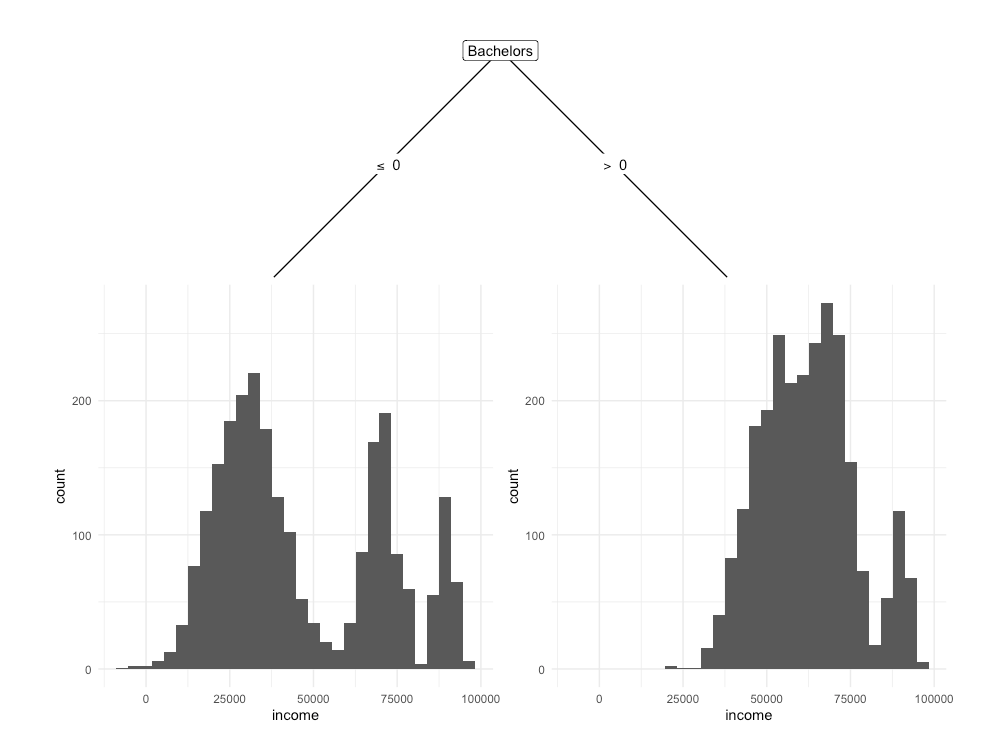
Decision trees can be used as a method for grouping units in a data set by asking questions, such as “Does an individual have a Bachelor’s degree?”. In this example, two groups would be created; one for those with a Bachelor’s degree, and one for those without. Figure 2 provides a visual depiction of this grouping in an attempt to explain Income.

Figure 4.1. Decision tree that splits units in a dataset based on whether individual has a Bachelor’s degree or not, in order to predict Income. The tree shows that those with a Bachelors degree (> 0) on average earn more than than those wihtout a Bachelor’s degree (< 0).

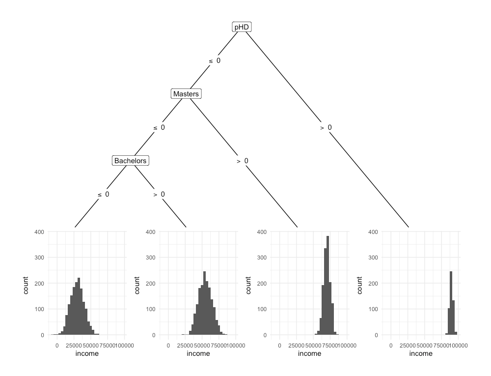
Each subsequent question in a decision tree will produce a smaller group of units. This grouping is carried out to identify units with similar characteristics with respect to an outcome variable. The model in Figure 3 attempts to use University qualifications to predict Income.

Figure 4.2. Decision tree that splits units in a dataset based on whether individual has a Bachelor’s degree (yes/no), a Master’s degree and PhD (yes/no), in order to predict Income. The tree shows that those with a higher qualification tend to earn more.

The following characteristics are true of decision trees:

• A single question is asked at each decision node, and there are only two possible choices. With the example in Figure 3, the questions include 1) Does the individual have a PhD, 2) Does the individual have a Master’s and 3) Does the individual have a Bachelor’s degree.
  
• At the bottom of every decision tree, there is a single possible decision. Every possible decision will eventually lead to a choice. Some decisions will lead to a choice sooner. The model in Figure 3 attempts to predict Income using University Qualifications. Each node presents a question about whether an individual possesses a given qualification. The end nodes present the distribution of income for individuals with the specified qualifications. As a result, the choices would be the expected value of Income for an individual, given the qualifications obtained.

Decision trees are a learning method that involve a tree like graph to model either continuous or categorical choice given some data. It is composed of a series of binary questions, which when answered in succession yield a prediction about data at hand. XGBoost uses Classification and Regression Trees (CART), which are presented in the above examples, to predict the outcome variable.

5.1.1 Boosting

A single decision tree is considered a weak/ base learner as it is only slightly better than chance at predicting the outcome variable. Whereas strong learners are any algorithm that can be tuned to achieve peak performance for supervised learning. XGBoost uses decision trees as base learners; combining many weak learners to form a strong learner. As a result it is referred to as an ensemble learning method; using the output of many models (i.e. trees) in the final prediction.

The concept of combining many weak learners to produce a strong learner is referred as boosting. XGBoost will iteratively build a set of weak models on subsets of the data; weighting each weak prediction according to the weak learner’s performance. A prediction is derived by taking the weighted sum of all base learners.

5.1.2 Building models with XGBoost

In the training data, a target variable \(y_{i}\) is specified, whilst all other features \(x_{i}\) are used as predictors of the target variable. A collection of decision trees are used to predict values of \(y_{i}\) using \(x_{i}\). Individually, each decision tree, would be a weak predictor of the outcome variable. However, as a collective, the decision trees may enable analysts to make accurate and reliable predictions of \(y_{i}\). The steps below demonstrate how XGBoost was used to build a model, to predict income, using University Qualifications.

1. Load the following packages

library(caret)

library(xgboost)

2. Load the data set and remove the identifier

# Load data
load("data/Income_tree.RData")

# Remove identifier
Income <- Income[,-1]

3. Split the data set into training and test

# Split data into training and test
set.seed(5)

s <- createDataPartition(Income$income, p = 0.8, list=FALSE)

training <- Income[s,]

test <- Income[-s,]

4. Convert the data into DMatrix objects, which is the recommended input type for xgboost

# Convert the data to matrix and assign output variable
train.outcome <- training$income

train.predictors <- sparse.model.matrix(income ~ .,
                                        data = training
)[, -1]

test.outcome <- test$income

test.predictors <- model.matrix(income ~ .,
                                data = test
)[, -1]

# Convert the matrix objects to DMatrix objects
dtrain <- xgb.DMatrix(train.predictors, label=train.outcome)

dtest <- xgb.DMatrix(test.predictors)

5. Train the model

# Train the model
model <- xgboost(
  data = dtrain, max_depth = 2, eta = 1, nthread = 2, nrounds = 10,
  objective = "reg:linear")

6. Test the model

# Test the model
pred <- predict(model, dtest)

# Evaluate the performance of model
RMSE(pred,test.outcome)

7. Examine the importance of each feature in the model

# Examine feature importance
importance_matrix <- xgb.importance(model = model)

print(importance_matrix)

xgb.plot.importance(importance_matrix = importance_matrix)

8. Plot the individual trees in the model

# Plot the trees
# Tree 1
xgb.plot.tree(model = model, tree=0)
# Tree 2
xgb.plot.tree(model = model, tree=1)
# Tree 3
xgb.plot.tree(model = model, tree=2)

5.2 An XGBoost Imputation pipeline

Two features of the XGBoost library that are relevant to highlight in the context of an imputation pipeline are:

• It can handle missingness in the predictory (or auxiliary) variables
  
• It can only carry out univariate prediction (or imputation)

Given those two features, the ideal method of productionising XGBoost in the context of imputation would be to:

1. Identify key outcome variables in the survey
   
2. Of variables selected in (1), identify those with a rate of missingness less than 40%
3. Build XGBoost models to predict each variable identified in (2) using all available auxiliary variables
   
4. Ensure that performance of XGBoost models in (3) meets requirements of clients
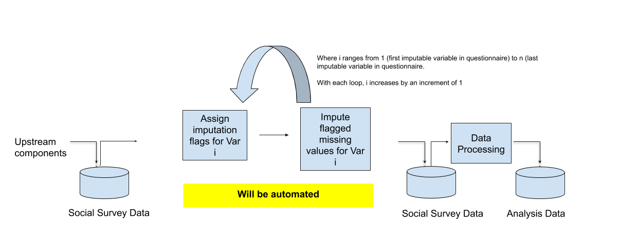
5. For all variables that have an approved model from (4), use a serial process to impute each variable, imputing them in the order in which they were presented to respondents

Figure 4.3 presents the proposed XGBoost imputation pipeline.

Figure 4.3. The proposed imputation pipeline using XGBoost.