Chapter 6 Methods
The project evaluated the machine learning methods using:
- The Census Teaching File, an open data set containing 1% of the person records from the 2011 Census in England & Wales.
- Survey Data
6.1 Data preparation
The following questions had to be answered when preparing the datasets for the imputation study:
How to treat categorical variables?
- As all methods required numeric data, categorical variables were either label or one hot encoded
- Readings suggested ensemble tree models perform better with label encoding. As a result, all variables were label encoded for evaluating XGBoost
- For neural networks, ordinal variables were label encoded, whereas nominal variables were one hot encoded
How to treat continuous variables with varying ranges?
- If there were multiple continuous variables in the dataset, with varying ranges, they were all normalised to have a mean of 0 and standard deviation of 1, for the model based methods. This was carried out to facilitate a more efficient search of the optimum parameters for the model based methods.
How to treat genuine missingness in the data (if present)?
- Instances where there was genuine item level missingness (i.e. cells that required imputation) were imputed with median (for continuous variables) or mode (for categorical variables) imputation
How to evaluate the generalisability of the methods?
- To evaluate how well the methods could be generalised, the dataset was split into a training set and a test set. The training set (80% of copmlete dataset) was used to make assumptions about the relationship between the auxiliary and imputable variables. Whereas the test (20% of copmlete dataset) was used to evaluate how well these assumptions generalise.
- Missingness was simulated in the test data to produce survey-like conditions. Missingness was simulated with varying rates for the auxiliary (up to 40% of cells) and imputable variables (50% of cells).
- To evaluate how well the methods could be generalised, the dataset was split into a training set and a test set. The training set (80% of copmlete dataset) was used to make assumptions about the relationship between the auxiliary and imputable variables. Whereas the test (20% of copmlete dataset) was used to evaluate how well these assumptions generalise.
How to treat the “no code required” (NCR) response classification for the imputable and auxiliary variables?
- All units with an NCR for the imputable variable were removed from the training and test set. As these cases could be deterministically imputed useing auxiliary variables, there was no need to train and evaluate the model with respect to how well it predicts the NCR cases for the imputable variable.
- Units with an NCR for the auxiliary variables were retained in the training and test set.
- All units with an NCR for the imputable variable were removed from the training and test set. As these cases could be deterministically imputed useing auxiliary variables, there was no need to train and evaluate the model with respect to how well it predicts the NCR cases for the imputable variable.
Figure 4 presents, at a high level, the methods used to prepare the dataset for this imputation study. It is important to note that a test dataset (with missingness) was created for each imputable variable. Specific details about data preparation, with respect to the Census teaching file and Survey data, are detailed below.
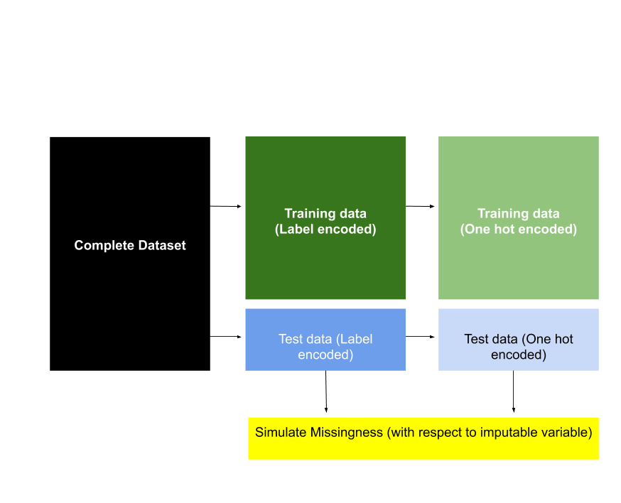
Figure 5.1. A high level overview of the methods used to create the training and test set for this imputation study
6.2 Census Teaching File
The Census Teaching File was downloaded from the ONS website as a CSV file named “CensusTeachingFile”, and was read into R using the following line of code. The data set consisted of 569,741 individuals and 18 categorical variables from the 2011 Census population.
# Read CSV into R
CensusRaw <- read.csv(
  file = "data/source/CensusTeachingFile.csv", skip = 1,
  header = TRUE, sep = ","
)
The code below specifies the packages used in the preparation, study and build of machine learning systems using the Census Teaching File.
library(tidyverse)
library(mice)
library(reshape2)
library(GGally)
library(Matrix)
library(xgboost)
library(caret)
library(DiagrammeR)
library(MLmetrics)
library(rpart)
library(scales)
library(knitr)
library(kableExtra)
library(DescTools)
library(dummies)
The steps below present the methods used to compare the performance of model based imputation (using XGBoost) with that of donor based imputation (using CANCEIS). Code chunks are provided to demonstrate how each step was carried out; with the imputable variable, economic activity, as the example. For a number of steps, functions were written, to standardise the process of preparing a dataset and evaluating imputaiton methods. Details of the functions used can be found in the appendix.
- Variables in the data set were renamed and recoded so that:
- Variable names were consistent with Google’s R style guide
- Label encoding was applied to all categorical variables
# Rename variables
Census <- plyr::rename(CensusRaw, c(
  "Person.ID" = "person.id",
  "Region" = "region",
  "Residence.Type" = "residence.type",
  "Family.Composition" = "fam.comp",
  "Population.Base" = "resident.type",
  "Sex" = "sex",
  "Age" = "age",
  "Marital.Status" = "marital.status",
  "Student" = "student",
  "Country.of.Birth" = "birth.country",
  "Health" = "health",
  "Ethnic.Group" = "ethnicity",
  "Religion" = "religion",
  "Economic.Activity" = "econ.act",
  "Occupation" = "occupation",
  "Industry" = "industry",
  "Hours.worked.per.week" = "hours.worked",
  "Approximated.Social.Grade" = "social.grade"
))

# Recode variables (dataset is mutated in order to recode variables)
Census <- Census %>% mutate_if(is.factor, as.character)

# Recode the Region variable so that it is numeric
Census$region[Census$region == "E12000001"] <- 1
Census$region[Census$region == "E12000002"] <- 2
Census$region[Census$region == "E12000003"] <- 3
Census$region[Census$region == "E12000004"] <- 4
Census$region[Census$region == "E12000005"] <- 5
Census$region[Census$region == "E12000006"] <- 6
Census$region[Census$region == "E12000007"] <- 7
Census$region[Census$region == "E12000008"] <- 8
Census$region[Census$region == "E12000009"] <- 9
Census$region[Census$region == "W92000004"] <- 10

Census$residence.type[Census$residence.type == "C"] <- 0
Census$residence.type[Census$residence.type == "H"] <- 1

Census$student[Census$student == 1] <- 0
Census$student[Census$student == 2] <- 1

Census$sex[Census$sex == 1] <- 0
Census$sex[Census$sex == 2] <- 1

Census$birth.country[Census$birth.country==1] <- 0
Census$birth.country[Census$birth.country==2] <- 1

Census <- Census %>% mutate_if(is.character, as.numeric)

Census$person.id <- as.character(Census$person.id)

Ht <- table(Census$hours.worked)
Census$hours.cont <- ifelse(Census$hours.worked == 1, runif(
  1:Ht[names(Ht) == 1],
  1, 15
),
ifelse(Census$hours.worked == 2, runif(1:Ht[names(Ht) == 2], 16, 30),
  ifelse(Census$hours.worked == 3, runif(1:Ht[names(Ht) == 3], 31, 48),
    ifelse(Census$hours.worked == 4, runif(1:Ht[names(Ht) == 4], 49, 60),
      Census$hours.worked
    )
  )
)
)

save(Census, file = "data/core/Census.Rda")

Census.pre.ohe <- Census

# Prepare Census data for one hot encoding
Census.pre.ohe$fam.comp[Census.pre.ohe$fam.comp == -9] <- "NCR"

Census.pre.ohe$health[Census.pre.ohe$health == -9] <- "NCR"

Census.pre.ohe$ethnicity[Census.pre.ohe$ethnicity == -9] <- "NCR"

Census.pre.ohe$religion[Census.pre.ohe$religion == -9] <- "NCR"

Census.pre.ohe$econ.act[Census.pre.ohe$econ.act == -9] <- "NCR"

Census.pre.ohe$occupation[Census.pre.ohe$occupation == -9] <- "NCR"

Census.pre.ohe$industry[Census.pre.ohe$industry == -9] <- "NCR"

Census.pre.ohe$social.grade[Census.pre.ohe$social.grade == -9] <- "NCR"
A preview of the data set is provided below.
| person.id | region | residence.type | fam.comp | resident.type | sex | age | marital.status | student | birth.country | health | ethnicity | religion | econ.act | occupation | industry | hours.worked | social.grade | hours.cont |
|---|---|---|---|---|---|---|---|---|---|---|---|---|---|---|---|---|---|---|
| 7394816 | 1 | 1 | 2 | 1 | 1 | 6 | 2 | 1 | 0 | 2 | 1 | 2 | 5 | 8 | 2 | -9 | 4 | -9.00000 |
| 7394745 | 1 | 1 | 5 | 1 | 0 | 4 | 1 | 1 | 0 | 1 | 1 | 2 | 1 | 8 | 6 | 4 | 3 | 52.97915 |
| 7395066 | 1 | 1 | 3 | 1 | 1 | 4 | 1 | 1 | 0 | 1 | 1 | 1 | 1 | 6 | 11 | 3 | 4 | 37.80685 |
| 7395329 | 1 | 1 | 3 | 1 | 1 | 2 | 1 | 1 | 0 | 2 | 1 | 2 | 1 | 7 | 7 | 3 | 2 | 39.52916 |
| 7394712 | 1 | 1 | 3 | 1 | 0 | 5 | 4 | 1 | 0 | 1 | 1 | 2 | 1 | 1 | 4 | 3 | 2 | 31.29265 |
| 7394750 | 1 | 1 | 2 | 1 | 0 | 6 | 2 | 1 | 0 | 2 | 1 | 1 | 1 | 9 | 2 | 3 | 3 | 31.04491 |
- Two versions of the dataset were created. One version applied label encoding for the categorical variables (created in step 1), whilst the other applied one hot encoding. The former was used when evaluating XGBoost; label encoding is generally recommended for ensemble tree models when there is high cardinality in the categorical variables (i.e. a large number of levels). The latter is intended to be used when evaluating neural networks.
Census_ohe <- dummy.data.frame(Census.pre.ohe,
  sep = ".",
  names = c(
    "region", "resident.type", "fam.comp",
    "marital.status", "health", "ethnicity",
    "religion", "econ.act", "occupation",
    "industry", "social.grade"
  )
)- For the purposes of training and testing a machine learning system, the data was divided into training and test data sets using the following code. Training and test versions of the dataset were created for both the label encoded and one hot encoded datasets.
# Randomly select 80% of Census units and split into Train and Test data
set.seed(5)
Census80 <- sample(1:nrow(Census_ohe), 0.8 * nrow(Census_ohe), replace = FALSE)
Census20 <- setdiff(1:nrow(Census_ohe), Census80)

Census.train.ohe <- Census_ohe[Census80, !(names(Census_ohe)=="hours.worked")]
Census.test.ohe <- Census_ohe[Census20, !(names(Census_ohe)=="hours.worked")]

Census.train.label <- Census[Census80, !(names(Census)=="hours.worked")]
Census.test.label <- Census[Census20, !(names(Census)=="hours.worked")]

save(Census.train.ohe, file = "data/ohe/Census.train.ohe.Rda")
save(Census.test.ohe, file = "data/ohe/Census.test.ohe.Rda")

save(Census.train.label, file = "data/label/Census.train.label.Rda")
save(Census.test.label, file = "data/label/Census.test.label.Rda")
The intention was to build models to predict a selection of variable using training data, which had no missingness. This model would then be evaluated with respect to its accuracy and generalisability using a test data set, which would have missingness. The Census Teaching File was a complete data set. As a result, missingness was simulated in the test data set, and the imputation models (derived for each variable) were evaluated with regards to how well they predicted the true values.
Models were tested for the following variables:
- Economic activity (a multi-class variable)
- Hours worked (a derived continuous variable)
- Social Grade (a multi-class variable)
- Student status (a binary variable)
A more detailed description of all the variables can be found here.
Each imputable variable had two test datasets:
- A version where one hot encoding was applied for the categorical auixilary variables
- A version where label encoding was applied for the categorical auxiliary variables
- Missingness was simulated in the test data using the functions “SimMissV”, and “LabelMiss”. The former simulates missingness in the one hot encoded dataset with respect to each imputable variable, and the latter maps this pattern of missingness to the label encoded dataset.
Each test dataset had the following mechanism and patterns of missingness:
- Mechanism: Missing at Random
Pattern:
- 40% of cells for the auxiliary variables were set to missing
- 50% of cells for imputable variable were set to missing
- 40% of cells for the auxiliary variables were set to missing
# With respect to variable 'EconAct'
Census.EconAct.ohe <- SimMissV(dat=Census.test.ohe,
                   ident = 'person.id',
                   var.aux = c('region','residence.type','fam.comp','resident.type',
                               'sex','age','marital.status','birth.country',
                               'health','ethnicity','religion','occupation','industry'),
                   ohe.vars = c('region','resident.type','fam.comp','marital.status',
                                'health','ethnicity','religion','econ.act','occupation',
                                'industry','social.grade'),
                   imp.vars = c('econ.act','hours.cont','social.grade','student'),
                   var = 'econ.act',
                   ohe = 1,
                   exc = 1,
                   drop = 'econ.act.NCR')

Census.EconAct.label <- LabelMiss(
  dat.label = Census.test.label,
  dat.ohe = Census.EconAct.ohe,
  ident = 'person.id',
  ohe_vars = c('region','resident.type','fam.comp','marital.status',
               'health','ethnicity','religion','econ.act','occupation',
               'industry','social.grade'),
  keep_var = c('person.id', 'region', 'residence.type', 'fam.comp', 'resident.type',
               'sex', 'age', 'marital.status', 'student', 'birth.country', 'health',
               'ethnicity', 'religion', 'econ.act', 'occupation', 'industry', 'hours.cont',
               'social.grade'))

save(Census.EconAct.ohe, file = "data/ohe/missingness/Census.EconAct.ohe.RData")

save(Census.EconAct.label, file = "data/label/missingness/Census.EconAct.label.RData")


# With respect to variable 'HoursCont'
Census.HoursCont.ohe <- SimMissV(dat=Census.test.ohe,
                                ident = 'person.id',
                                var.aux = c('region','residence.type','fam.comp','resident.type',
                                            'sex','age','marital.status','birth.country',
                                            'health','ethnicity','religion','occupation','industry'),
                                ohe.vars = c('region','resident.type','fam.comp','marital.status',
                                             'health','ethnicity','religion','econ.act','occupation',
                                             'industry','social.grade'),
                                imp.vars = c('econ.act','hours.cont','social.grade','student'),
                                var = 'hours.cont',
                                ohe = 0,
                                exc = -9)

Census.HoursCont.label <- LabelMiss(
  dat.label = Census.test.label,
  dat.ohe = Census.HoursCont.ohe,
  ident = 'person.id',
  ohe_vars = c('region','resident.type','fam.comp','marital.status',
               'health','ethnicity','religion','econ.act','occupation',
               'industry','social.grade'),
  keep_var = c('person.id', 'region', 'residence.type', 'fam.comp', 'resident.type',
               'sex', 'age', 'marital.status', 'student', 'birth.country', 'health',
               'ethnicity', 'religion', 'econ.act', 'occupation', 'industry', 'hours.cont',
               'social.grade'))

save(Census.HoursCont.ohe, file = "data/ohe/missingness/Census.HoursCont.ohe.RData")

save(Census.HoursCont.label, file = "data/label/missingness/Census.HoursCont.label.RData")

# With respect to variable 'SocialGrade'
Census.SocialGrade.ohe <- SimMissV(dat=Census.test.ohe,
                                  ident = 'person.id',
                                  var.aux = c('region','residence.type','fam.comp','resident.type',
                                              'sex','age','marital.status','birth.country',
                                              'health','ethnicity','religion','occupation','industry'),
                                  ohe.vars = c('region','resident.type','fam.comp','marital.status',
                                               'health','ethnicity','religion','econ.act','occupation',
                                               'industry','social.grade'),
                                  imp.vars = c('econ.act','hours.cont','social.grade','student'),
                                  var = 'social.grade',
                                  ohe = 1,
                                  exc = 1,
                                  drop = 'social.grade.NCR')

Census.SocialGrade.label <- LabelMiss(
  dat.label = Census.test.label,
  dat.ohe = Census.SocialGrade.ohe,
  ident = 'person.id',
  ohe_vars = c('region','resident.type','fam.comp','marital.status',
               'health','ethnicity','religion','econ.act','occupation',
               'industry','social.grade'),
  keep_var = c('person.id', 'region', 'residence.type', 'fam.comp', 'resident.type',
               'sex', 'age', 'marital.status', 'student', 'birth.country', 'health',
               'ethnicity', 'religion', 'econ.act', 'occupation', 'industry', 'hours.cont',
               'social.grade'))

save(Census.SocialGrade.ohe, file = "data/ohe/missingness/Census.SocialGrade.ohe.RData")

save(Census.SocialGrade.label, file = "data/label/missingness/Census.SocialGrade.label.RData")

# With respect to variable 'Student'
Census.Student.ohe <- SimMissV(dat=Census.test.ohe,
                                  ident = 'person.id',
                                  var.aux = c('region','residence.type','fam.comp','resident.type',
                                              'sex','age','marital.status','birth.country',
                                              'health','ethnicity','religion','occupation','industry'),
                                  ohe.vars = c('region','resident.type','fam.comp','marital.status',
                                               'health','ethnicity','religion','econ.act','occupation',
                                               'industry','social.grade'),
                                  imp.vars = c('econ.act','hours.cont','social.grade','student'),
                                  var = 'student',
                                  ohe = 0,
                                  exc = -9)

Census.Student.label <- LabelMiss(
  dat.label = Census.test.label,
  dat.ohe = Census.Student.ohe,
  ident = 'person.id',
  ohe_vars = c('region','resident.type','fam.comp','marital.status',
               'health','ethnicity','religion','econ.act','occupation',
               'industry','social.grade'),
  keep_var = c('person.id', 'region', 'residence.type', 'fam.comp', 'resident.type',
               'sex', 'age', 'marital.status', 'student', 'birth.country', 'health',
               'ethnicity', 'religion', 'econ.act', 'occupation', 'industry', 'hours.cont',
               'social.grade'))

save(Census.Student.ohe, file = "data/ohe/missingness/Census.Student.ohe.RData")

save(Census.Student.label, file = "data/label/missingness/Census.Student.label.RData")- The distribution of the imputable variable was studied
# Study the variable: How many units in each category?
EAt <- table(Census$econ.act)

EAt

# What is the distribution of the variable: Remove NCR and plot to look at distribution
g <- ggplot(Census[!Census$econ.act == -9, ], aes(econ.act))

g + geom_bar() + scale_x_discrete(
  name = "Economic Activity",
  breaks = pretty_breaks()
)- An XGBoost model was built using the training set
econAct <- trainDT(
  train = Census.train.label,
  test.orig = Census.test.label,
  test.miss = Census.EconAct.label,
  ident = 'person.id',
  cat = 1,
  var = 'econ.act',
  exc = -9,
  col_order = c("region", "residence.type", "fam.comp", "resident.type", "sex",
                "age", "marital.status", "student", "birth.country", "health", "ethnicity",
                "religion", "econ.act", "occupation", "industry", "social.grade", "hours.cont"),
  objective = "multi:softmax",
  max_depth = 5,
  eta = 0.3,
  nrounds = 30,
  num_class = 10
)
Donor based imputation was carried out on the test data:
- CANCEIS: One round of CANCEIS selected matching variables based on a correlation matrix. Variables that were most closely related to the imputable variable were selected as matching variables in the CANCEIS imputation specification. As all variables were categorical (or in the case of hours worked had a categorical equivalent), Goodman and Kurskall’s Lambda was used as a measure of how strong the relationship between the variables were. The four auxiliary variables with the highest Labmda score were selected as matching variables. And weights were assigned to correspond with the Labmda measure; higher scores meant variables were assigned a greater weight. The function “CANCEIS.in” was used to select the matching variables.
- Mixed Methods: One round of CANCEIS selected matching variables based on the feature importance figures from the XGBoost model; focusing on the cover measure for the variables. The six most important variables from the feature importance output were selected as matching variables; with more important variables assigned a larger weight. The function “CANCEISXG” was used to select the matching variables.
- CANCEIS: One round of CANCEIS selected matching variables based on a correlation matrix. Variables that were most closely related to the imputable variable were selected as matching variables in the CANCEIS imputation specification. As all variables were categorical (or in the case of hours worked had a categorical equivalent), Goodman and Kurskall’s Lambda was used as a measure of how strong the relationship between the variables were. The four auxiliary variables with the highest Labmda score were selected as matching variables. And weights were assigned to correspond with the Labmda measure; higher scores meant variables were assigned a greater weight. The function “CANCEIS.in” was used to select the matching variables.
econAct.CANCEIS <- CANCEIS.in(
  dat.cor=Census,
  dat.miss=Census.EconAct.label,
  var='econ.act',
  exc=-9,
  varlist=c("region", "residence.type", "fam.comp", "resident.type", "sex",
            "age", "marital.status", "student", "birth.country", "health", "ethnicity",
            "religion", "econ.act", "occupation", "industry", "social.grade", "hours.worked"))

write.table(econAct.CANCEIS[[2]],
            file = "data/CANCEIS/EconAct/xxxUNIT01IG01.txt", sep = "\t",
            row.names = FALSE, col.names = FALSE
)
# Impute values using CANCEIS (with XGBoost to advise selection of MVs)
# Create CANCEIS input file with imputable and matching variables
econAct.CANCEISXG <- CANCEISXG(
dat.miss = Census.EconAct.label,
var = 'econ.act',
featureList = econAct[[3]])
write.table(econAct.CANCEISXG[[1]],
file = "data/CANCEISXG/EconAct/xxxUNIT01IG01.txt", sep = "\t",
row.names = FALSE, col.names = FALSE
)- Evaluate the performance of XGBoost, CANCEIS and Mixed Methods imputation. The following performance metrics were used:
Continuous variables
- Root mean squared error
- Mean absolute error
- Root mean squared error
Categorical variables
- Accuracy
- Cohen’s Kappa
- Accuracy
Figures were also produced to demonstrate the performance of each method. A plot of the confusion matrix indicated how well each level of the categorical imputable variables were predicted. Whilst a distribution of the variables post imputation relative to the actual distribution was used to demonstrate how well the imputed dataset mapped the actual distribution of the imputable variable.
# Save feature importance plot
png(filename="images/featuresXG_econAct.png")
xgb.plot.importance(importance_matrix = econAct[[3]])
dev.off()

# Examine quality metrics
compareMissing <- econAct[[7]]

counts <- table(compareMissing$indicator)

counts.melt <- melt(counts)

counts.melt$Outcome <- counts.melt$Var1

accuracy_plot <- ggplot(data=counts.melt, aes(x=Outcome, y=value)) +
  geom_bar(stat="identity") + ggtitle("Accuracy of Predictions: XGBoost")

accuracy_plot

ggsave("images/accuracyXG_econAct.png")

confusion_XGBoost <- confusionMatrix(
  factor(compareMissing$Actuals, levels = 1:9),
  factor(compareMissing$Predictions, levels = 1:9)
)

qplot(Actuals, Predictions,
      data = compareMissing,
      geom = c("jitter"), main = "XGBoost: predicted vs. observed in test data",
      xlab = "Observed Class", ylab = "Predicted Class"
) + scale_x_discrete(limits=c("1","2","3","4","5","6","7","8","9")
) + scale_y_discrete(limits=c("1","2","3","4","5","6","7","8","9"))

ggsave("images/EAXGBoostqplot.png")

# What is the distribution of the variable before and after imputation
Compare_val <- econAct[[6]]

actuals <- ggplot(econAct[[6]], aes(Actuals))

actuals + geom_bar() + ggtitle("True Distribution") +
  scale_x_discrete(
    name = "Economic Activity",
    breaks = pretty_breaks()
  )

ggsave("images/actuals_socialGrade.png")

actuals <- table(Compare_val$Actuals)

actuals <- as.data.frame(actuals)

actuals <- plyr::rename(actuals, c(
  "Var1" = "econ.act",
  "Freq" = "actuals"))

imputed <- table(Compare_val$PI)

imputed <- as.data.frame(imputed)

imputed <- plyr::rename(imputed, c(
  "Var1" = "econ.act",
  "Freq" = "imputed"))

plot.dat <- merge(actuals, imputed, by = "econ.act")

plot.dat.melt <- melt(plot.dat, id="econ.act")

plot.dat.melt <- plyr::rename(plot.dat.melt, c(
  "variable" = "output"))

predictions <- ggplot(plot.dat.melt, aes(x=econ.act,y=value,fill=output)) +
  geom_bar(stat="identity", position = "identity", alpha=.5)

predictions + ggtitle("Post Imputation: XGBoost") +
  scale_x_discrete(
    name = "Economic Activity",
    breaks = pretty_breaks()
  )

ggsave("images/PIXG_econAct.png")

# Save model
trainEA_v1 <- econAct[[2]]

xgb.save(trainEA_v1, "models/XGBoost/xgboost.econAct")

# Save predicted values
predicted.econAct <- econAct[[5]]

save(predicted.econAct, file = "data/predicted/XGBoost/predicted.econAct.RData")
# Load CANCEIS input and output files
econAct.CANCEIS.load <- loadCANCEIS(
var='EconAct',
varlist=names(econAct.CANCEIS[[2]]),
xg=0)
eval.econAct.CANCEIS <- evalCANCEIS(cat=1,
var = 'econ.act',
exc = -9,
actuals = Census.test.label,
missing = econAct.CANCEIS.load[[1]],
predicted = econAct.CANCEIS.load[[2]],
matchkey = econAct.CANCEIS[[3]])
# Compare predicted and actuals
counts <- eval.econAct.CANCEIS[[3]]
counts.melt <- melt(counts)
counts.melt$Outcome <- counts.melt$Var1
accuracy_plot <- ggplot(data=counts.melt, aes(x=Outcome, y=value)) +
geom_bar(stat="identity") + ggtitle("Accuracy of Predictions: CANCEIS")
accuracy_plot
ggsave("images/accuracyCANCEIS_econAct.png")
# Using Confusion Matrix to evaluate predictions
compareMissing_CANCEIS <- eval.econAct.CANCEIS[[2]]
confusion_CANCEIS <- confusionMatrix(
factor(compareMissing_CANCEIS$Actuals, levels = 1:9),
factor(compareMissing_CANCEIS$Predictions, levels = 1:9)
)
qplot(Actuals, Predictions,
data = compareMissing_CANCEIS,
geom = c("jitter"), main = "CANCEIS: predicted vs. observed in test data",
xlab = "Observed Class", ylab = "Predicted Class"
) + scale_x_discrete(limits=c("1","2","3","4","5","6","7","8","9")
) + scale_y_discrete(limits=c("1","2","3","4","5","6","7","8","9"))
ggsave("images/EACANCEISqplot.png")
# What is the distribution of the variable after imputation?
Compare_val <- eval.econAct.CANCEIS[[1]]
actuals <- table(Compare_val$Actuals)
actuals <- as.data.frame(actuals)
actuals <- plyr::rename(actuals, c(
"Var1" = "econ.act",
"Freq" = "actuals"))
imputed <- table(Compare_val$Predictions)
imputed <- as.data.frame(imputed)
imputed <- plyr::rename(imputed, c(
"Var1" = "econ.act",
"Freq" = "imputed"))
plot.dat <- merge(actuals, imputed, by = "econ.act")
plot.dat.melt <- melt(plot.dat, id="econ.act")
plot.dat.melt <- plyr::rename(plot.dat.melt, c(
"variable" = "output"))
predictions <- ggplot(plot.dat.melt, aes(x=econ.act,y=value,fill=output)) +
geom_bar(stat="identity", position = "identity", alpha=.5)
predictions + ggtitle("Post Imputation: CANCEIS") +
scale_x_discrete(
name = "Economic Activity",
breaks = pretty_breaks()
)
ggsave("images/PICANCEIS_econAct.png")# Load CANCEIS input and output files
econAct.CANCEISXG.load <- loadCANCEIS(
var='EconAct',
varlist=names(econAct.CANCEISXG[[1]]),
xg=1)
eval.econAct.CANCEISXG <- evalCANCEIS(
cat =1,
var = 'econ.act',
exc = -9,
actuals = Census.test.label,
missing = econAct.CANCEISXG.load[[1]],
predicted = econAct.CANCEISXG.load[[2]],
matchkey = econAct.CANCEISXG[[2]])
# Compare predicted and actuals
counts <- eval.econAct.CANCEISXG[[3]]
counts.melt <- melt(counts)
counts.melt$Outcome <- counts.melt$Var1
accuracy_plot <- ggplot(data=counts.melt, aes(x=Outcome, y=value)) +
geom_bar(stat="identity") + ggtitle("Accuracy of Predictions: CANCEISXG")
accuracy_plot
ggsave("images/accuracyCANCEISXG_econAct.png")
# Using Confusion Matrix to evaluate predictions
compareMissing_CANCEISXG <- eval.econAct.CANCEISXG[[2]]
confusion_CANCEISXG <- confusionMatrix(
factor(compareMissing_CANCEISXG$Actuals, levels = 1:9),
factor(compareMissing_CANCEISXG$Predictions, levels = 1:9)
)
qplot(Actuals, Predictions,
data = compareMissing_CANCEISXG,
geom = c("jitter"), main = "predicted vs. observed in test data",
xlab = "Observed Class", ylab = "Predicted Class"
) + scale_x_discrete(limits=c("1","2","3","4","5","6","7","8","9")
) + scale_y_discrete(limits=c("1","2","3","4","5","6","7","8","9"))
ggsave("images/EACANCEISXGqplot.png")
# What is the distribution of the variable after imputation?
Compare_val <- eval.econAct.CANCEISXG[[1]]
actuals <- table(Compare_val$Actuals)
actuals <- as.data.frame(actuals)
actuals <- plyr::rename(actuals, c(
"Var1" = "econ.act",
"Freq" = "actuals"))
imputed <- table(Compare_val$Predictions)
imputed <- as.data.frame(imputed)
imputed <- plyr::rename(imputed, c(
"Var1" = "econ.act",
"Freq" = "imputed"))
plot.dat <- merge(actuals, imputed, by = "econ.act")
plot.dat.melt <- melt(plot.dat, id="econ.act")
plot.dat.melt <- plyr::rename(plot.dat.melt, c(
"variable" = "output"))
predictions <- ggplot(plot.dat.melt, aes(x=econ.act,y=value,fill=output)) +
geom_bar(stat="identity", position = "identity", alpha=.5)
predictions + ggtitle("Post Imputation: CANCEISXG") +
scale_x_discrete(
name = "Economic Activity",
breaks = pretty_breaks()
)
ggsave("images/PICANCEISXG_econAct.png")