Chapter 5 Text Analysis Tools Part 3, Topic Modelling
In this section, we will explore another strategy for analyzing text data: topic modelling! Topically, we will focus our analyses on water rights along the Colorado River.
5.1 Water Rights Along the Colorado River
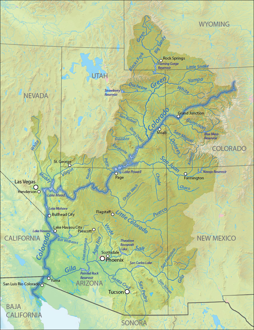
The Colorado River Basin is mainly fed by snow pack in the Rocky Mountains, and provides water to 36 million people across seven Western states (Arizona, California, Colorado, Nevada, New Mexico, Texas, and Utah). The full river basin includes many tributaries, and two major dams (Lake Powell and Lake Mead).
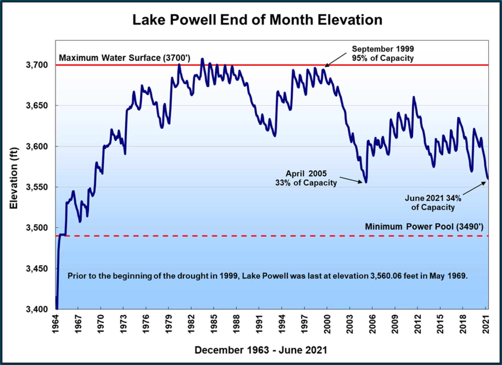
Currently, the water levels at both Lake Powell and Lake Meed are critically low. The following chart shows water levels at Lake Powell, which was filled in the early 1970’s and has been depleted in recent decades by increasing populations and agriculture usage in the West, droughts, and rising temperatures.
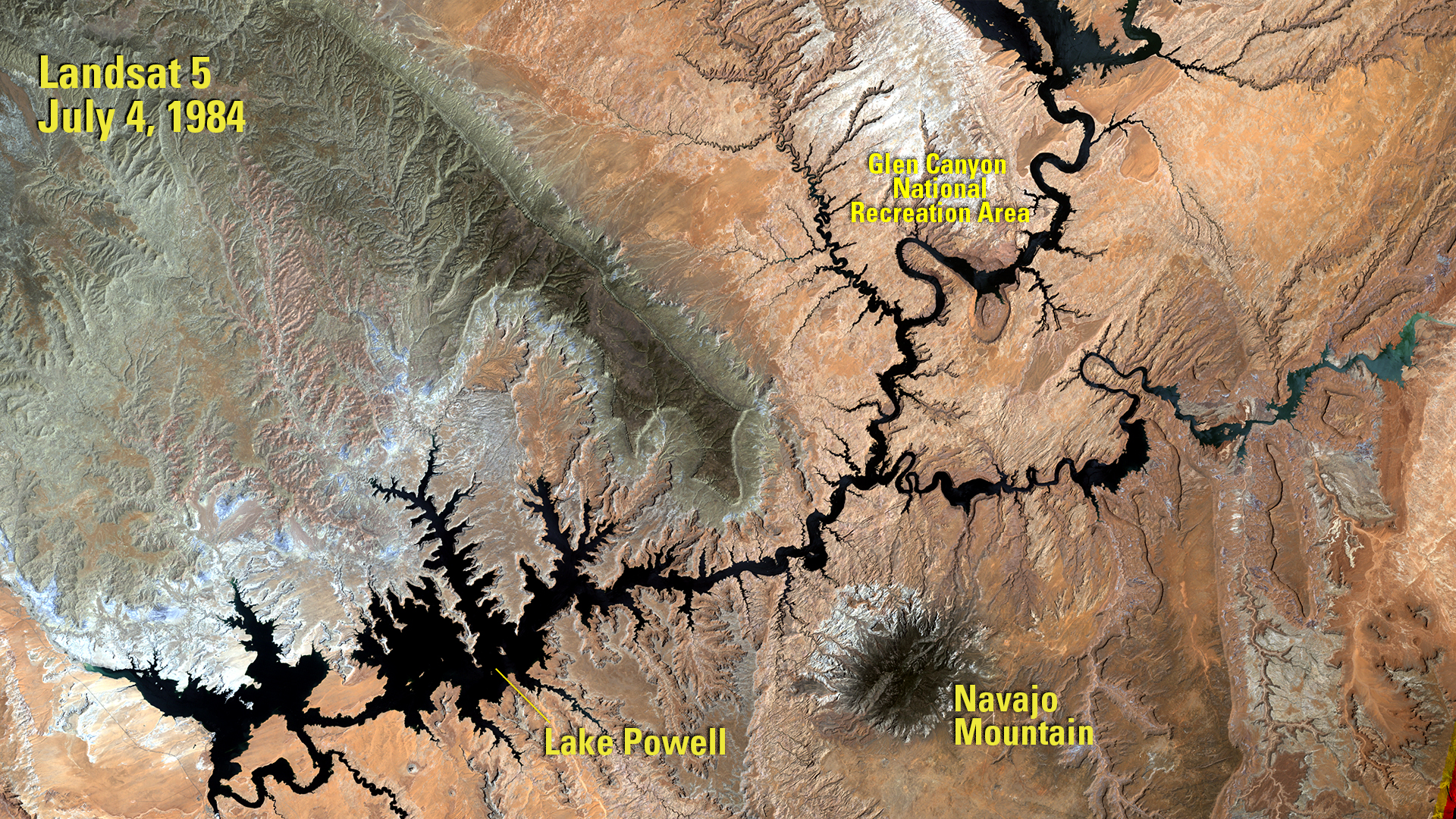
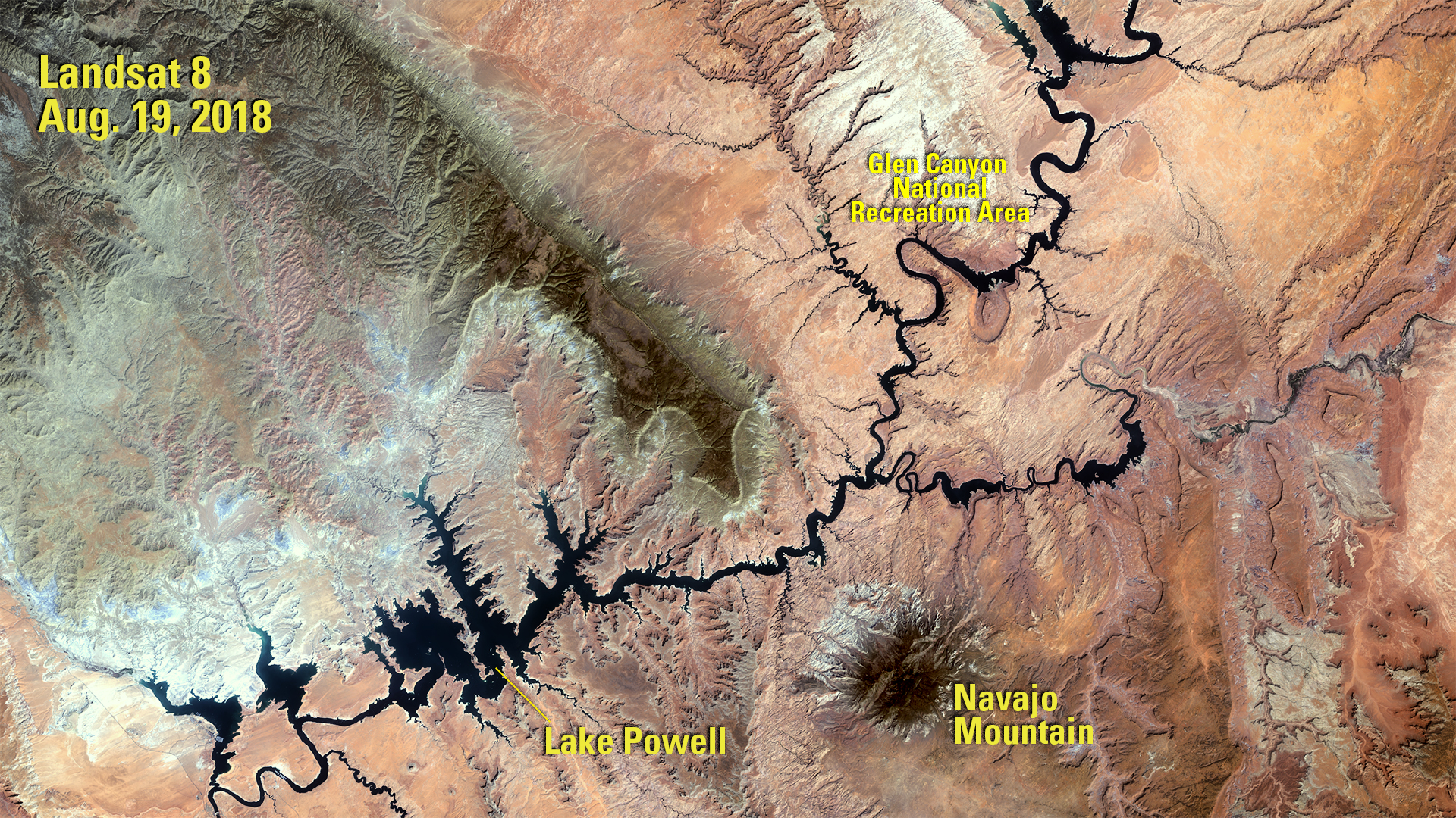
We can see this depletion by looking at satellite images:
In Wendy Espeland’s book The Struggle For Water, she describes the negotiations and politics among government actors and Native tribes at the heart of the Central Arizona Project, a proposed dam that would help provide water for millions but also destroy vast amounts of wildlife and infringe upon Native people’s sovereignty. She explores themes of tension and politics as various groups, including the “Old Guard” and “New Guard” at the Bureau of Reclamation, and the Yavapai people. Each of these groups bring a separate set of rationalities into water management, which are often at odds with each other, and from which we can learn about bureaucratic organizations and resource management in the current age.
For the purposes of this class, we will look at news stories about the Colorado River to examine themes of resource management. Specifically, we will search for all Guardian articles that mention the river:
We end up with 351 articles spanning dates between 1999 and 2023. I’ve uploaded these data on Canvas as “guardian_co_river.csv.”
5.2 What is Topic Modelling?
Topic modelling is an “unsupervised” method for sorting text data into groups. That is, there are no correct topics that the model is trying to identify. Rather, the model sorts words and documents according to some criteria, and we can adjust these depending on how well it is doing.
Let’s first get our Guardian data in tidytext format.
library(dplyr)
library(tidytext)

# create a tidytext dataset
tidy_co <- co_river %>%
  unnest_tokens(word, body_text) %>%
  anti_join(stop_words)
We will now count the words in each article separately. Including id inside the count() parentheses does this.
# create counts of each word - we will include id in the count()
# function to also get n values for words in each article
tidy_co_counts <- tidy_co %>%
  count(id, word, sort = TRUE)
Great! Now, to run topic models on our data, we need to put it into a Document-Term Matrix (DTM). The DTM is similar to other tidytext data that we have used, but there are some characteristics that make the DTM unique. Silge and Robinson note that in the DTM:
- Each row represents a document.
- Each variable represents a term.
- Each value contains the number of appearances of the term.
We might intuit that when we create a DTM with many documents and many terms, there will be a large number of 0’s (terms that do not appear in specific documents). This is especially the case when terms are specific and documents are relatively short (for example, we might have songs with different lyrics in each, and many words would appear rarely). When a dataframe or matrix has a low frequency of non-zero values, we call it sparse.
Perfect! Now we have a DTM object that is essentially a matrix with the value of appearances for each word in each document (0’s for most entries).
The method of topic modelling that we will use is called “Latent Dirichlet Allocation,” or LDA. It is the most common form of topic modelling. LDA treats documents as “mixtures” of topics, and topics as “mixtures” of words. Importantly, each of these can be overlapping, such that words can appear in multiple topics and topics can appear in multiple documents.
We can calculate LDA in R using the following code. Importantly, we need to specify the number of topics that we want to use. We’ll start here with two topics, but it’s wise to try different numbers and look at the results under each scenario. Since this is unsupervised learning, remember that there is no “correct” answer, but that some will be better than others. We will also use the control argument to set a seed equal to 1, so that we get the same result every time (otherwise, it could give us a slightly different LDA).
Great! Now that we have a topic model for our data, we just need to get it into a format that we can work with. The tidy() function, as its name suggests, gives us a tidy dataframe. When we input an LDA object into the tidy() function, it gives us \(\beta\) values, which represent the probability that a given word will fall into a given topic. You may need to install the package reshape2 for this code to work:
Now that our data are in a tidy dataframe, we’ll just clean it up a little more so that we can plot it. We will keep the top ten words in each topic, and sort them by their \(\beta\) values.
# format for plot
co_top_terms <- co_topics %>%
  group_by(topic) %>%
  slice_max(beta, n = 10) %>%
  ungroup() %>%
  arrange(topic, -beta) %>%
  mutate(term = reorder_within(term, beta, topic))
And lastly, we will plot the topics.
library(ggplot2)
# plot our topics!
ggplot(co_top_terms, aes(beta, term, fill = factor(topic))) +
geom_col(show.legend = FALSE) +
facet_wrap(~ topic, scales = "free") +
scale_y_reordered()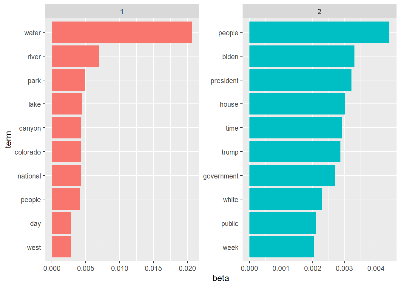
If we were to label these topics, what we we call them?
Alternatively, we could try plotting the topics in relation to each other. That is, we can take \(log\bigg(\frac{\beta_2}{\beta_1}\bigg)\) to compare the \(\beta\) values for the same word in two different topics. Then we can look at the ten words that are relatively most common in each topic. We will also filter our data to only include words that have \(\beta\) values above 0.001 in at least one topic.
library(tidyr)
beta_wide <- co_topics %>%
  mutate(topic = paste0("topic", topic)) %>%
  pivot_wider(names_from = topic, values_from = beta) %>%
  filter(topic1 > .001 | topic2 > .001) %>%
  mutate(log_ratio = log2(topic2 / topic1))
For plotting purposes, we will limit our data to the 10 largest and smallest log ratio values. We will do this by re-assigning beta_wide using the bind_rows() function with two arguments: beta_wide limited to the largest 10 values, and beta_wide limited to the smallest ten values. For each dataframe, we will add a variable called “topic,” which we will call “topic1” for the smallest values (since these are most likely to appear in topic 1) and “topic2” for the largest values (since these are more likely to appear in topic 2).
# limit to 10 largest and smallest log ratios
beta_wide <- bind_rows(
  beta_wide %>%
    slice_min(log_ratio, n = 10) %>%
    mutate(topic = "topic1"),
  beta_wide %>%
    slice_max(log_ratio, n = 10) %>%
    mutate(topic = "topic2")
)
Now we can plot our result!
# plot results!
ggplot(beta_wide, aes(x = log_ratio, y = term))+
  geom_col()+
  facet_grid(rows = vars(topic), scales = "free_y")+
  labs(x = "Log Ratio", y = "Term")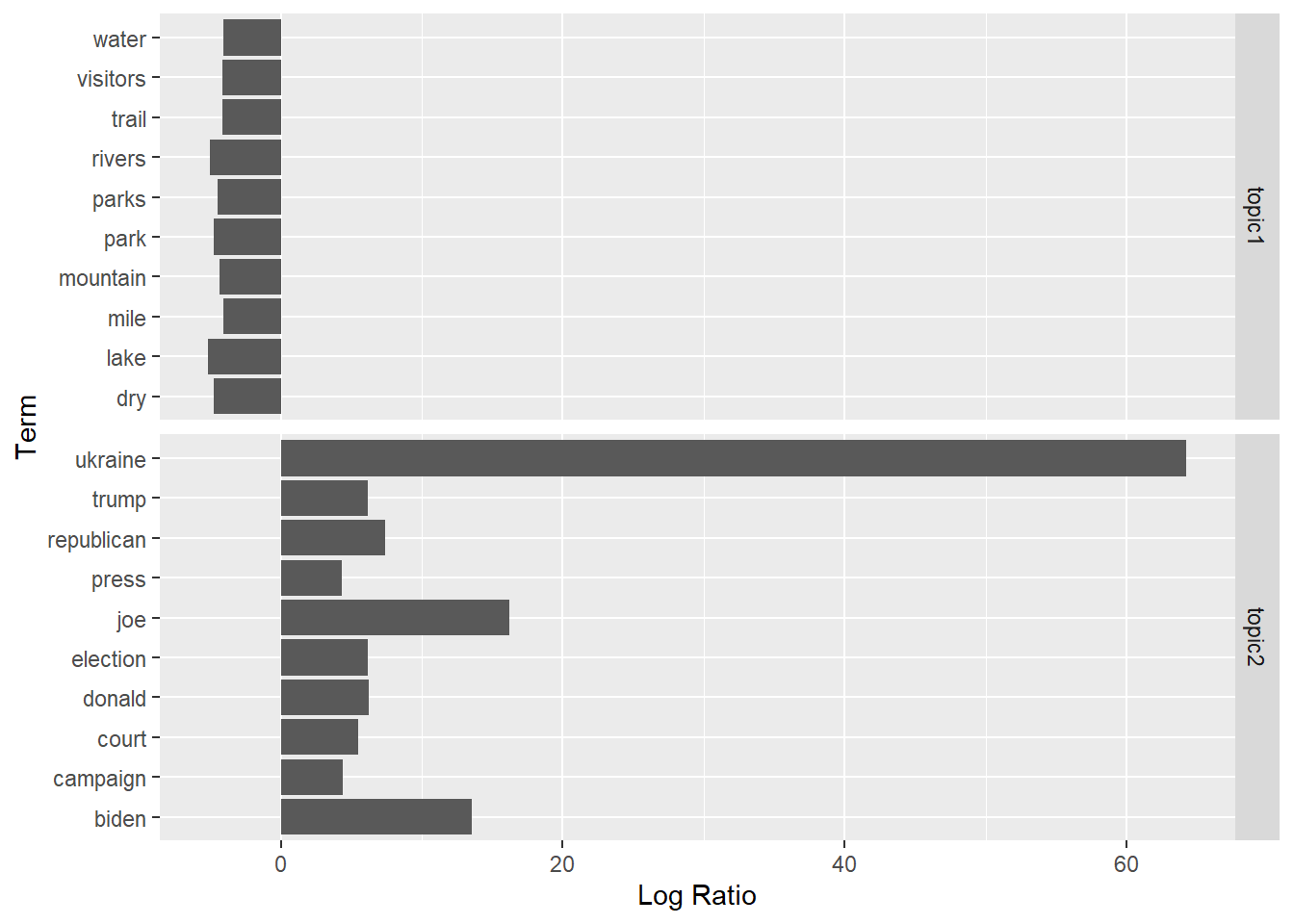
Great! From here, we can more clearly see the divide between Topic 1 and Topic 2. We could even label our topics: for example, “Nature” and “Politics.” These labels aren’t perfect, but they roughly describe the sets of words that appear in each broad category.
5.3 Documents as Mixtures of Topics
Until now, we have mostly been examining topics as mixtures of words. It makes sense to do this as an initial step: we want to see that our topics can be understood as broad categories and that the words classified under these topics have something in common. But we could also move up a level, examining documents as mixtures of topics.
Here, we are asking what topics our documents - in this case, Guardian news articles - are comprised of. We can do this by calculating the \(\gamma\) for the LDA.\(\gamma\) can be interpreted as the “per-document-per-topic probabilities,” which add to 1 for each document. We can think of these as the proportion of each topic within a document.
# calculate gamma for all documents
co_documents <- tidy(co_lda, matrix = "gamma")

# view documents
head(co_documents)
## # A tibble: 6 × 3
## document topic gamma
## <chr> <int> <dbl>
## 1 global-development/2013/jul/06/water-supplies-shrinking-threat-… 1 1.00e+0
## 2 world/live/2023/jun/20/russia-ukraine-war-live-attacks-reported… 1 2.70e-5
## 3 film/2023/feb/21/herzog-swinton-rushdie-cinema-tom-luddy-tellur… 1 8.57e-1
## 4 environment/2018/may/25/best-us-national-parks-escape-crowds 1 1.00e+0
## 5 us-news/2016/apr/25/drought-water-rights-wet-asset-buying-snake… 1 9.39e-1
## 6 sustainable-business/blog/us-water-paradox-demand-infrastructure 1 1.00e+0Within co_documents, we can search for specific articles and find the topics that they are comprised of. For example:
# examine one article
co_documents %>%
  filter(document == "world/uselectionroadtrip/2008/oct/17/uselections2008")
## # A tibble: 2 × 3
## document topic gamma
## <chr> <int> <dbl>
## 1 world/uselectionroadtrip/2008/oct/17/uselections2008 1 0.478
## 2 world/uselectionroadtrip/2008/oct/17/uselections2008 2 0.522We see that this article is roughly evenly between the two topics. If we look at the article, we can see that it is about the presidential campaign trail in 2008, but specifically about Obama’s campaign Arizona. The article describes the desert scenery while also conveying the significance of the region to the unfolding presidential race. Therefore, it makes sense that this article is split roughly evenly between the “nature” and “politics” topics.
As a contrast, let’s take a look at the articles that most strongly align with just one topic. Specifically, we’ll look at articles that have probabilities of greater than 95% for one topic.
## # A tibble: 224 × 3
##    document                                                          topic gamma
##    <chr>                                                             <int> <dbl>
##  1 global-development/2013/jul/06/water-supplies-shrinking-threat-t…     1 1.00
##  2 environment/2018/may/25/best-us-national-parks-escape-crowds          1 1.00
##  3 sustainable-business/blog/us-water-paradox-demand-infrastructure      1 1.00
##  4 artanddesign/2017/feb/23/cut-in-two-travels-along-the-us-mexico-…     1 0.952
##  5 environment/2015/may/17/lake-powell-drought-colorado-river            1 1.00
##  6 global/2023/may/31/arizona-farmers-water-colorado-river-cuts          1 1.00
##  7 environment/2018/nov/20/national-parks-america-overcrowding-cris…     1 1.00
##  8 travel/2015/jan/19/top-10-long-distance-hiking-trails-us-califor…     1 1.00
##  9 travel/2016/aug/24/10-least-visited-us-national-parks                 1 1.00
## 10 us-news/2023/feb/16/great-salt-lake-disappear-utah-poison-climat…     1 0.965
## # ℹ 214 more rows
Wow, 224 articles! As it turns out, the vast majority of our Guardian articles are about “nature” rather than “politics.”
5.4 Choosing \(k\) Values
Perhaps the most important decision we can make in topic modelling is the \(k\) value for our model. If \(k\) is too large, we’ll end up with a lot of topics that don’t make any sense, and if \(k\) is too small, we’ll end up with lots of different themes in the same topics. While one can inductively explore various options, there are also formalized ways to search for optimal \(k\) values.
Regardless of our method for choosing \(k\), we should always make sure that our models align with our human validation of what topics make sense. That is, we shouldn’t rely solely on our output metrics to make decisions about our data, we should also incorporate the knowledge that we have about our sources and our goals.
There are a few ways that we can search for optimal \(k\) values. We’ll start by looking at the FindTopicsNumber function from the ldatuning package. We’ll try searching for topics within the range of 2-20, and using two methods - (Cao & Juan, 2009) and (Devaud, 2014). The package includes two other methods - (Griffiths, 2004) and (arun, 2010) - which you may want to inspect as well, especially if there is uncertainty between the first two.
library(ldatuning)

# create models with different number of topics
result <- ldatuning::FindTopicsNumber(
  co_dtm,
  topics = seq(from = 2, to = 20, by = 1),
  metrics = c("CaoJuan2009",  "Deveaud2014"),
  method = "Gibbs",
  control = list(seed = 3),
  verbose = TRUE
)
## fit models... done.
## calculate metrics:
## CaoJuan2009... done.
## Deveaud2014... done.The ldatuning package also includes a function for visualizing the results:
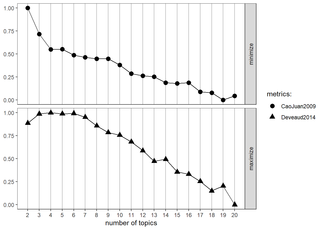
As noted in the above figure, we want to minimize the (Cao, Juan 2009) estimator while maximizing the (Deveaud, 2014) estimator. Therefore, we might want to explore running our models with 4 topics, as well as 6, 14, and 19. From this point, we would want to re-run our topic models at this values and manually inspect the results. In the Problem Set, you’ll have a chance to try 4 topics.
Lastly, I want to note that Structural Topic Models are an alternative to LDA, which incorporate article-level metadata in their topic modelling. The stm R package has many wonderful features for text processing, finding topics, and creating visualizations. I recommend exploring this vignette if you wish to deepen your understanding of topic models!
5.5 Problem Set 5
Recommended Resources:
Text Mining with R: A Tidy Approach
An Introduction to Topic Modelling
Run a topic model with 4 topics on the “guardian_co_river.csv” dataset.
Plot the top words for each topic, similar to what is done in section 5.2. What would you label these topics?
Try running the LDA again, this time with a different number of topics. Does the new topic model make more or less sense to you?
Using whichever topic model made the most sense to you, create a dataset similar to
co_documentsin section 5.3. Choose two articles to examine in more detail. Discuss the topic probabilities.Considering what we know about the Colorado River and water rights in the U.S. (from readings and class), are we surprised by the topics generated by these news articles? Describe how your results compared to expectations.