3 Ridge Regression
3.1 Introduction
Ridge regression was proposed as an alternative method to ordinary least squares (OLS), that trades bias for variance to improve the mean square error (\(MSE\)).
\(MSE\big(\hat{\beta}\big) = var \big(\hat{\beta}\big) + \underbrace{\left(\mathbb E\big(\hat{\beta}\big)-\beta \right)^2}_{bias^2}\)
This method is particularly useful when the \(OLS\) is unstable (high variance). This can happen in presence of high collinearity between the predictors or when the number of predictors is large in comparison to the number of observations.
The ridge estimator is obtained by maximising the likelihood with a restriction. This equivalent to minimising the residual sum of squares with an added penalisation term.
\(\underbrace{\sum^{n}_{i=1} \left(y_i-\beta_0-\sum^{p}_{j=1} \beta_j x_{ij}\right)^2 }_{\text {residual sum of squares}}+ \lambda \underbrace{\sum^{p}_{j=1} \beta_j^2}_{\ell_2-penalisation}\)
This is called a \(\ell_2\) penalisation, because is based on the \(\ell_2\) norm, \(\| \beta \|_2 = \sqrt{\sum_{j=1}^p \beta_j^2}\). The amount of penalisation is controlled by a parameter (\(\lambda\)). This parameter can be estimated by cross-validation. Basically, is finding the \(\lambda\) that gives the optimal trade-off between bias and variance to minimise the \(MSE\).
3.3 Practical session
Task 1 - Fit a linear model with Ridge penalisation
We will use the fat dataset in the library(faraway). We want to compare the OLS and Ridge estimates of a linear model to predict body fat (variable brozek), using the other variables available, except for siri , density and free .
Let’s first read the data
#install.packages(c("glmnet", "faraway"))
library(glmnet)   #function for ridge regression
library(faraway) #has the dataset fat
set.seed(1233)data("fat")
head(fat)## brozek siri density age weight height adipos free neck chest abdom hip
## 1 12.6 12.3 1.0708 23 154.25 67.75 23.7 134.9 36.2 93.1 85.2 94.5
## 2 6.9 6.1 1.0853 22 173.25 72.25 23.4 161.3 38.5 93.6 83.0 98.7
## 3 24.6 25.3 1.0414 22 154.00 66.25 24.7 116.0 34.0 95.8 87.9 99.2
## 4 10.9 10.4 1.0751 26 184.75 72.25 24.9 164.7 37.4 101.8 86.4 101.2
## 5 27.8 28.7 1.0340 24 184.25 71.25 25.6 133.1 34.4 97.3 100.0 101.9
## 6 20.6 20.9 1.0502 24 210.25 74.75 26.5 167.0 39.0 104.5 94.4 107.8
## thigh knee ankle biceps forearm wrist
## 1 59.0 37.3 21.9 32.0 27.4 17.1
## 2 58.7 37.3 23.4 30.5 28.9 18.2
## 3 59.6 38.9 24.0 28.8 25.2 16.6
## 4 60.1 37.3 22.8 32.4 29.4 18.2
## 5 63.2 42.2 24.0 32.2 27.7 17.7
## 6 66.0 42.0 25.6 35.7 30.6 18.8We will first fit the linear regression using ridge.
The package glmnet implements the ridge estimation.
We need to define the design matrix of the model, \(X\) and identify
the outcome \(Y\)
############################################################
#RIDGE REGRESSION
############################################################

#we need to define the model equation
X <- model.matrix(brozek ~  age + weight +
                    height + adipos +
                    neck + chest +
                    abdom + hip + thigh +
                    knee + ankle +
                    biceps + forearm +
                    wrist, data=fat)[,-1]
#and the outcome
Y <- fat[,"brozek"]
First we need to find the amount of penalty, \(\lambda\) by cross-validation. We will search for the \(\lambda\) that give the minimum \(MSE\) in the interval
\(\lambda = \exp(-5)= 0.007\) to \(\lambda = \exp(8)= 2981\)
The function cv.glmnet() fits a glm using penalisation. alpha = 0
gets the ridge estimates for different levels of penalisation. The \(\lambda\)
chosen by cross-validation is stored in lambda.min.
#Penalty type (alpha=0 is ridge)
  cv.lambda <- cv.glmnet(x=X, y=Y,
                        alpha = 0,
                        lambda=exp(seq(-5,8,.1)))  #don't need to specify the range
                                                   #but you can do it anyways

  plot(cv.lambda)                                 #MSE for several lambdas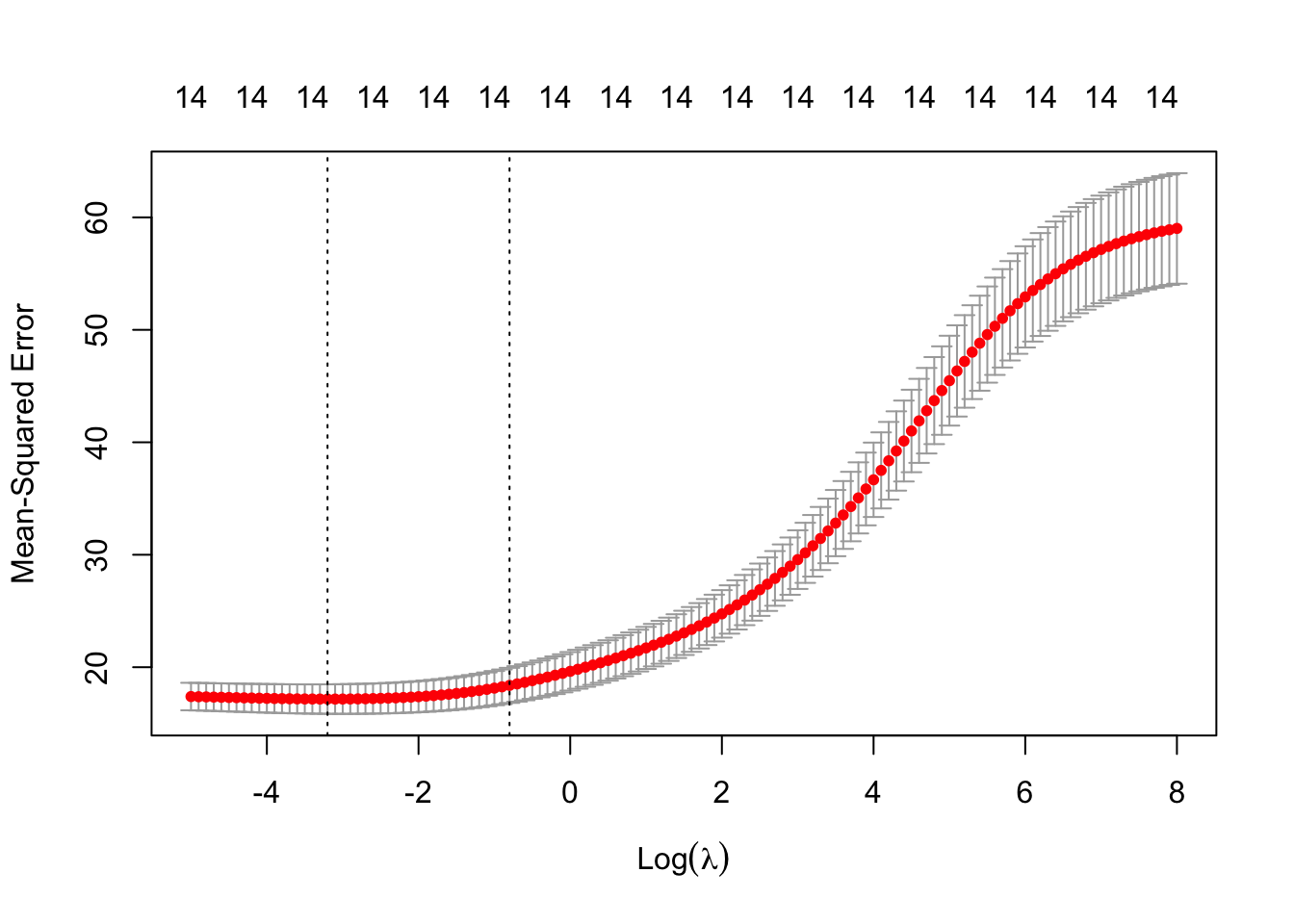
cv.lambda$lambda.min #best lambda## [1] 0.0407622The minimum \(MSE\) is achieved when \(\lambda =\) 0.0407622.
We can also see the impact of different \(\lambda\)s in the estimated coefficients. When \(\lambda\) is very high, the coefficients are shrunk towards zero.
#ridge path
  plot(cv.lambda$glmnet.fit,
       "lambda", label=FALSE)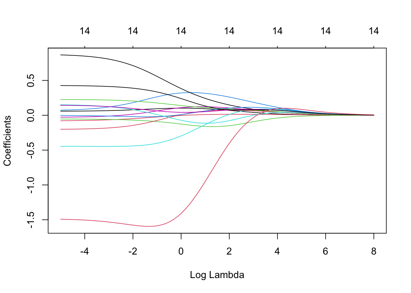
With the chosen \(\lambda =\) 0.0407622, we can now obtain the ridge estimates:
#now get the coefs with
#the lambda found above
  lmin        <- cv.lambda$lambda.min
  ridge.model <- glmnet(x=X, y=Y,
                        alpha = 0,
                        lambda = lmin)
  ridge.model$beta
## 14 x 1 sparse Matrix of class "dgCMatrix"
## s0
## age 0.06507401
## weight -0.06789165
## height -0.06028540
## adipos 0.10207562
## neck -0.45063815
## chest -0.01601489
## abdom 0.81945358
## hip -0.18402114
## thigh 0.22019252
## knee -0.01128917
## ankle 0.12891779
## biceps 0.13023719
## forearm 0.41741050
## wrist -1.51553984And finally, compare them with the OLS. Notice that in this case, the coefficients are similar because the penalisation was low.
  ols.regression <- lm(brozek ~  age + weight +                 #OLS
                         height + adipos +
                         neck + chest +
                         abdom + hip + thigh +
                         knee + ankle +
                         biceps + forearm +
                         wrist, data=fat)
  #OLS vs RIDGE
  round(cbind(OLS = coef(ols.regression),
        ridge = c(ridge.model$a0,                              #intercept for
                  as.vector(ridge.model$beta))),4)             #ridge
## OLS ridge
## (Intercept) -15.1901 -13.0910
## age 0.0569 0.0651
## weight -0.0813 -0.0679
## height -0.0531 -0.0603
## adipos 0.0610 0.1021
## neck -0.4450 -0.4506
## chest -0.0309 -0.0160
## abdom 0.8790 0.8195
## hip -0.2031 -0.1840
## thigh 0.2274 0.2202
## knee -0.0010 -0.0113
## ankle 0.1572 0.1289
## biceps 0.1485 0.1302
## forearm 0.4297 0.4174
## wrist -1.4793 -1.5155Task 2 - Ridge logistic model
With the lowbwt.csv dataset, in the library(faraway), we want to fit a ridge logistic regression to predict low birthweight (<2500gr), using age, lwt, race, smoke, ptl, ht, ui, ftv.
Let’s read the data and make sure that race and ftv are factor predictors. And recode ftv into (0, 1, 2+)
library(glmnet)lowbwt <- read.csv("https://www.dropbox.com/s/1odxxsbwd5anjs8/lowbwt.csv?dl=1",
stringsAsFactors = TRUE)
lowbwt$race <- factor(lowbwt$race,
levels = c(1,2,3),
labels = c("White", "Black", "Other"))
#number of previous appointments
lowbwt$ftv[lowbwt$ftv>1] <- 2 #categories 0, 1, 2+
lowbwt$ftv <- factor(lowbwt$ftv,
levels = c(0,1,2),
labels = c("0", "1", "2+"))
head(lowbwt)## id low age lwt race smoke ptl ht ui ftv bwt
## 1 85 0 19 182 Black 0 0 0 1 0 2523
## 2 86 0 33 155 Other 0 0 0 0 2+ 2551
## 3 87 0 20 105 White 1 0 0 0 1 2557
## 4 88 0 21 108 White 1 0 0 1 2+ 2594
## 5 89 0 18 107 White 1 0 0 1 0 2600
## 6 91 0 21 124 Other 0 0 0 0 0 2622Let’s first get the MLE estimates for the model for low using all the predictors.
lowbwt.logit <- glm(low ~ age +
                      lwt + race +
                      smoke + ptl +
                      ht + ui + ftv,
                    family=binomial, data=lowbwt)
summary(lowbwt.logit)
##
## Call:
## glm(formula = low ~ age + lwt + race + smoke + ptl + ht + ui +
## ftv, family = binomial, data = lowbwt)
##
## Deviance Residuals:
## Min 1Q Median 3Q Max
## -1.9907 -0.8247 -0.5154 0.9791 2.1624
##
## Coefficients:
## Estimate Std. Error z value Pr(>|z|)
## (Intercept) 0.590930 1.213568 0.487 0.62630
## age -0.026945 0.037414 -0.720 0.47141
## lwt -0.015748 0.006963 -2.262 0.02371 *
## raceBlack 1.254016 0.529382 2.369 0.01784 *
## raceOther 0.820827 0.451042 1.820 0.06878 .
## smoke 0.865245 0.414450 2.088 0.03683 *
## ptl 0.604607 0.357445 1.691 0.09075 .
## ht 1.894689 0.705977 2.684 0.00728 **
## ui 0.732822 0.460442 1.592 0.11148
## ftv1 -0.299057 0.463918 -0.645 0.51917
## ftv2+ 0.178370 0.450777 0.396 0.69233
## ---
## Signif. codes: 0 '***' 0.001 '**' 0.01 '*' 0.05 '.' 0.1 ' ' 1
##
## (Dispersion parameter for binomial family taken to be 1)
##
## Null deviance: 234.67 on 188 degrees of freedom
## Residual deviance: 200.61 on 178 degrees of freedom
## AIC: 222.61
##
## Number of Fisher Scoring iterations: 4We will use cv.glmnet() to find the best \(\lambda\)
lowbwt.complete <- lowbwt[complete.cases(lowbwt), ]

#we need to define the model equation
X.low <- model.matrix(low ~  age +
                      lwt + race +
                      smoke + ptl +
                      ht + ui + ftv,
                  data=lowbwt.complete)[,-1]
#and the outcome
Y.low <- lowbwt[,"low"]

cv.lambda <- cv.glmnet(x=X.low, y=Y.low,
                       alpha = 0,
                       family = binomial
                       )

plot(cv.lambda) 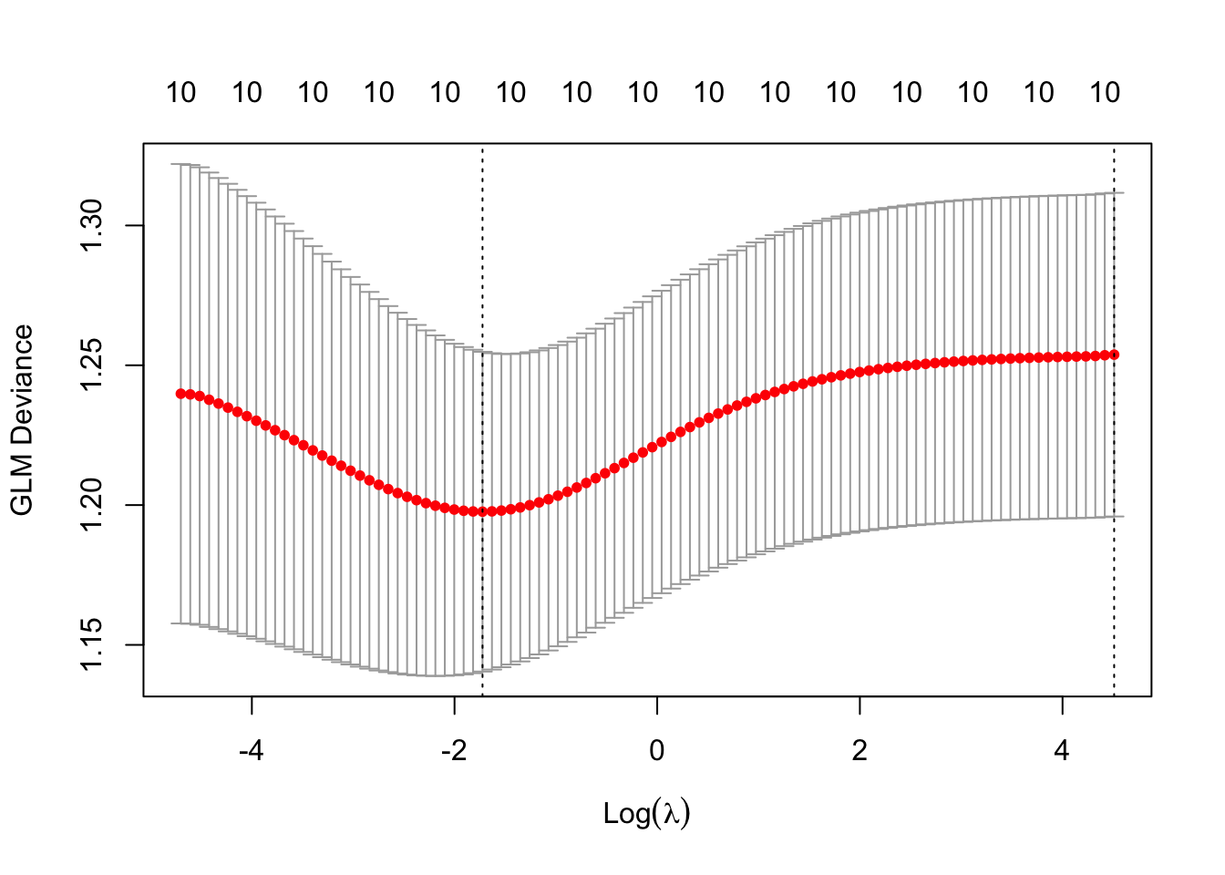
cv.lambda$lambda.min ## [1] 0.178367lmin <- cv.lambda$lambda.minAnd now use the chosen \(\lambda\) we can get the ridge estimates.
ridge.model <- glmnet(x=X.low, y=Y.low,
                        alpha = 0,
                        family = binomial,
                        lambda = lmin)
ridge.model$beta
## 10 x 1 sparse Matrix of class "dgCMatrix"
## s0
## age -0.01894794
## lwt -0.00647133
## raceBlack 0.44325516
## raceOther 0.27673349
## smoke 0.36274052
## ptl 0.37692639
## ht 0.84447200
## ui 0.43631641
## ftv1 -0.21840476
## ftv2+ -0.01265976TRY IT YOURSELF:
- Plot the ridge path
See the solution code
plot(cv.lambda$glmnet.fit, xvar="lambda")
- What would you get if we used a
lambda = 0in theglmnet()function?
See the solution code
#The estimates would be the same as the MLE
#obtained with the glm()
ridge.model <- glmnet(x=X.low, y=Y.low,
                        alpha = 0,
                        family = binomial,
                        lambda = .04)
ridge.model$beta
3.4 Exercises
Solve the following exercise:
The dataset lowbwt.csv has the birth weigh of 189 newborns and information about the mother’s pregnancy.
Fita linear model to predict birth weight (variable bwt) using all other predictors except for low and id. Get the ridge estimates and compare the coefficients with the OLS.
See the solution code
library(glmnet)
set.seed(2100)

#read the data

bwt.data <- read.csv("https://www.dropbox.com/s/1odxxsbwd5anjs8/lowbwt.csv?dl=1",
                   stringsAsFactors = TRUE)
bwt.data$race <- factor(bwt.data$race,
                      levels = c(1,2,3),
                      labels = c("White", "Black", "Other"))
head(bwt.data)


#Fit the OLS linear model
OLS.bwt <- lm (bwt ~ age+race+
                smoke+ptl+ht+ui+ftv,
                data = bwt.data)
summary(OLS.bwt)

#  Define the model
X <- model.matrix(bwt ~ age+
                    race+smoke+
                    ptl+ht+ui+ftv,
                  data = bwt.data)[, -1]
Y <- bwt.data[, "bwt"]

#Let's find the lambda  by cross-validation with that gives the minimum MSE

cv.lambda <- cv.glmnet(x=X, y=Y,
                       alpha = 0,
                       type.measure = "mse",        #adding type.measure="mse"
                       lambda = exp(seq(-6,8,0.1))) #will plot the lambda vs MSE
plot(cv.lambda)
cv.lambda$lambda.min

#he minimum MSE if when the lambda = 0.033

#  path diagram
plot(cv.lambda$glmnet.fit, "lambda", label = FALSE)

# with the  lambda that achieves the minimum MSE we can now obtain the ridge estimates
lmin <- cv.lambda$lambda.min
ridge.model <- glmnet(x=X, y=Y,
                      alpha = 0,
                      lambda = lmin)
ridge.model$beta

# Compare the ridge estimates with the OLS estimates
round(cbind(OLS = coef(OLS.bwt),
            ridge = c(ridge.model$a0, as.vector(ridge.model$beta))), 4)
The dataset
prostatea variable in the packagefarawaycontains information on 97 men who were about to receive a radical prostatectomy. These data come from a study examining the correlation between the prostate specific antigen (lpsa) and a number of other clinical measures.Fit the ridge estimators for linear model to predict lpsa using all other predictors. Plot the path diagram.
See the solution code
library(faraway)
library(glmnet)
set.seed(2000)
data("prostate")
head(prostate)


#  Define the model
X <- model.matrix(lpsa ~ lcavol + lweight +
                    age + lbph + svi+
                    lcp + gleason + pgg45,
                  data = prostate)[, -1]
Y <- prostate[, "lpsa"]

#Let's find the lambda  by cross-validation with that gives the minimum MSE

cv.lambda <- cv.glmnet(x=X, y=Y,
                       alpha = 0,
                       lambda = exp(seq(-6,8,0.1)))
plot(cv.lambda)
cv.lambda$lambda.min

#he minimum MSE if when the lambda = 0.033

#  path diagram
plot(cv.lambda$glmnet.fit, "lambda", label = FALSE)

# with the  lambda that achieves the minimum MSE we can now obtain the ridge estimates
lmin <- cv.lambda$lambda.min
ridge.model <- glmnet(x=X, y=Y,
                      alpha = 0,
                      lambda = lmin)
ridge.model$beta

# Compare the ridge estimates with the OLS estimates
ols.lm <- lm(lpsa ~ ., data = prostate)
round(cbind(OLS = coef(ols.lm),
            ridge = c(ridge.model$a0, as.vector(ridge.model$beta))), 4)
The \(\lambda\) penalty that was used is very close to 0, therefore the ridge estimates are similar to the OLS
- Fit the same model as in 2) but with high penalisation value (high lambda). What was the impact in the coefficients?
See the solution code
library(lasso2)
library(glmnet)
set.seed(2000)
data("prostate")
head(prostate)

#  Define the model (this is the same as the model in 2)
X <- model.matrix(lpsa ~ lcavol +
                    lweight + age +
                    lbph + svi+
                    lcp + gleason +
                    pgg45,
                  data = prostate)[, -1]
Y <- prostate[, "lpsa"]

# ridge estimates for high lambda (e.g, lambda=15)

ridge.model2 <- glmnet(x=X, y=Y,
                       alpha = 0,
                       lambda = 15 )
ridge.model2$beta

# Step 4) Compare the ridge estimates with the OLS estimates
ols.lm <- lm(lpsa ~ ., data = prostate)
round(cbind(OLS = coef(ols.lm),
            ridge = c(ridge.model$a0, as.vector(ridge.model2$beta))), 4)
The coefficients get shrunk towards 0 but they don’t reach 0!