4 Lasso Regression
4.1 Introduction
With Ridge regression we introduced the idea of penalisation that could result in estimators with smaller \(MSE\), benefiting from a bias-variance trade-off in the estimation process.
The penalisation in ridge regression shrinks the estimators towards 0. However, due to the nature of the penalisation, the estimators never reach zero no matter how much penalisation we introduce.
The Lasso uses a similar idea as ridge, but it uses a \(\ell_1\) penalisation (\(\ell_1\) norm is given by \(\mid \beta \mid= \sqrt{\sum^{p}_{n=1}\mid \beta_j \mid}\) ), that allows the coefficients to shrink exactly to 0.
This way, the estimation process has embedded a variable selection procedure, because if a coefficient shrinks to 0, it is the same as removing the variable from the model
To get the Lasso estimates we have to minimise:
\(\sum^{n}_{i=1} \left(y_i-\beta_0-\sum^{p}_{j=1} \beta_j x_{ij}\right)^2 + \lambda \underbrace{\sum^{p}_{j=1} \mid{\beta_j}\mid}_{\ell^1-penalisation}\)
Similar to ridge regression, the amount of penalisation is controlled by the parameter (\(\lambda\)) than can be chosen by cross-validation.
One important aspect that it is not discussed in the book, is the current limitation of Lasso regarding conventional inference. Computing the p-values or confidence intervals for the coefficients of a model fitted with lasso, remains an open problem.
4.3 Practical session
Task 1 - Fit a linear model with Lasso
We will use the fat dataset in the library(faraway). We want to use Lasso to select the best predictors for body fat (variable brozek), using the other variables available, except for siri , density and free .
Let’s first read the data
#install.packages(c("glmnet", "faraway"))
library(glmnet)   #function for ridge regression
library(faraway) #has the dataset fat
set.seed(1233)data("fat")
head(fat)## brozek siri density age weight height adipos free neck chest abdom hip
## 1 12.6 12.3 1.0708 23 154.25 67.75 23.7 134.9 36.2 93.1 85.2 94.5
## 2 6.9 6.1 1.0853 22 173.25 72.25 23.4 161.3 38.5 93.6 83.0 98.7
## 3 24.6 25.3 1.0414 22 154.00 66.25 24.7 116.0 34.0 95.8 87.9 99.2
## 4 10.9 10.4 1.0751 26 184.75 72.25 24.9 164.7 37.4 101.8 86.4 101.2
## 5 27.8 28.7 1.0340 24 184.25 71.25 25.6 133.1 34.4 97.3 100.0 101.9
## 6 20.6 20.9 1.0502 24 210.25 74.75 26.5 167.0 39.0 104.5 94.4 107.8
## thigh knee ankle biceps forearm wrist
## 1 59.0 37.3 21.9 32.0 27.4 17.1
## 2 58.7 37.3 23.4 30.5 28.9 18.2
## 3 59.6 38.9 24.0 28.8 25.2 16.6
## 4 60.1 37.3 22.8 32.4 29.4 18.2
## 5 63.2 42.2 24.0 32.2 27.7 17.7
## 6 66.0 42.0 25.6 35.7 30.6 18.8We will use package glmnet to fit the linear regression with lasso.
As in ridge regression, we need to define the design matrix of the model,
\(X\) and identify the outcome \(Y\)
############################################################
#LASSO REGRESSION
############################################################
#install.packages("glmnet")
library(glmnet)
set.seed(1233)

#we need to define the model equation
  X <- model.matrix(brozek ~  age + weight +
                      height + adipos +
                      neck + chest +
                      abdom + hip + thigh +
                      knee + ankle +
                      biceps + forearm +
                      wrist, data=fat)[,-1]
#and the outcome
  Y <- fat[,"brozek"]
First we need to find the amount of penalty, \(\lambda\) by cross-validation. We will search for the \(\lambda\) that give the minimum \(MSE\).
#Penalty type (alpha=1 is lasso
#and alpha=0 is the ridge)
  cv.lambda.lasso <- cv.glmnet(x=X, y=Y,
                         alpha = 1)
  plot(cv.lambda.lasso)                        #MSE for several lambdas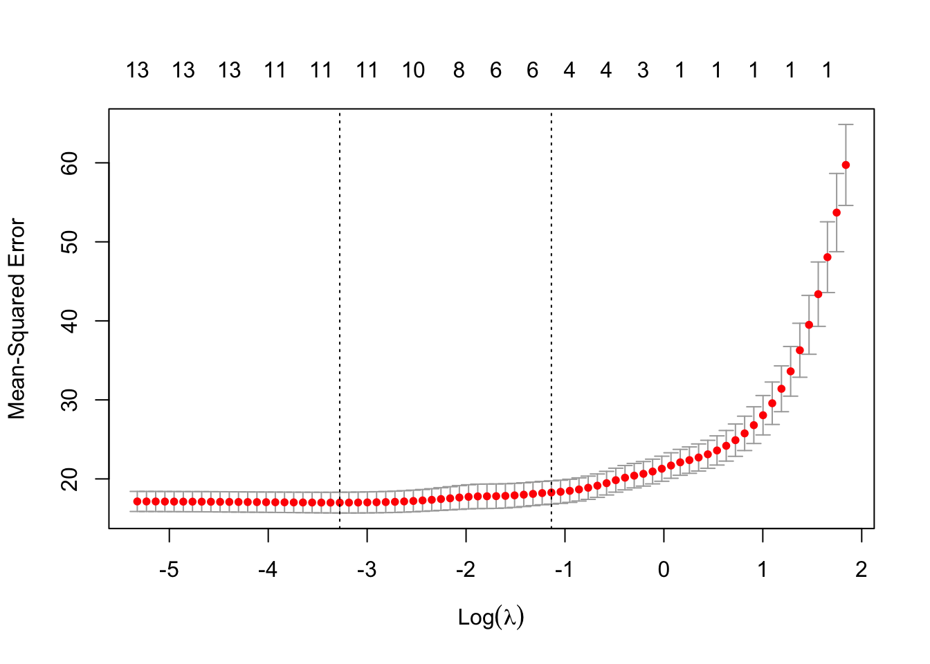
cv.lambda.lasso #best lambda##
## Call: cv.glmnet(x = X, y = Y, alpha = 1)
##
## Measure: Mean-Squared Error
##
## Lambda Index Measure SE Nonzero
## min 0.0377 56 17.00 1.314 11
## 1se 0.3206 33 18.28 1.471 4The minimum \(MSE\) is achieved when \(\lambda =\) 0.0377339.
We can also see the impact of different \(\lambda\)s in the estimated coefficients. When \(\lambda\) is very high, all the coefficients are shrunk exactly to zero.
#Lasso path
plot(cv.lambda.lasso$glmnet.fit,
     "lambda", label=FALSE)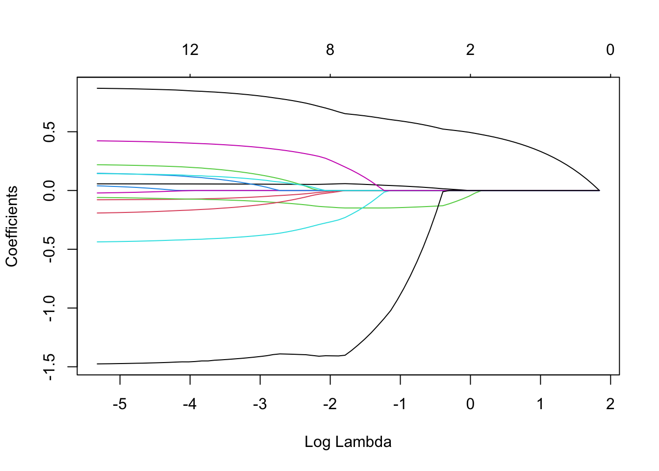
With the chosen \(\lambda =\) 0.0377339, we can now obtain the lasso estimates:
#now get the coefs with
#the lambda found above
l.lasso.min <- cv.lambda.lasso$lambda.min
lasso.model <- glmnet(x=X, y=Y,
                      alpha  = 1,
                      lambda = l.lasso.min)
lasso.model$beta                               #Coefficients
## 14 x 1 sparse Matrix of class "dgCMatrix"
## s0
## age 0.05425763
## weight -0.06183557
## height -0.08489983
## adipos .
## neck -0.39543236
## chest .
## abdom 0.82234754
## hip -0.13782057
## thigh 0.15795430
## knee .
## ankle 0.06991538
## biceps 0.10540827
## forearm 0.38050109
## wrist -1.42248095And finally, compare them with the OLS Notice that in this case, the coefficients are similar because the penalisation was low.
ols.model <- glm(brozek ~  age + weight +
                          height + adipos +
                          neck + chest +
                          abdom + hip + thigh +
                          knee + ankle +
                          biceps + forearm +
                          wrist, data=fat)

summary(ols.model)
##
## Call:
## glm(formula = brozek ~ age + weight + height + adipos + neck +
## chest + abdom + hip + thigh + knee + ankle + biceps + forearm +
## wrist, data = fat)
##
## Deviance Residuals:
## Min 1Q Median 3Q Max
## -10.2573 -2.5919 -0.1031 2.9040 9.2754
##
## Coefficients:
## Estimate Std. Error t value Pr(>|t|)
## (Intercept) -1.519e+01 1.611e+01 -0.943 0.3467
## age 5.688e-02 3.003e-02 1.894 0.0594 .
## weight -8.130e-02 4.989e-02 -1.630 0.1045
## height -5.307e-02 1.034e-01 -0.513 0.6084
## adipos 6.101e-02 2.780e-01 0.219 0.8265
## neck -4.450e-01 2.184e-01 -2.037 0.0427 *
## chest -3.087e-02 9.779e-02 -0.316 0.7526
## abdom 8.790e-01 8.545e-02 10.286 <2e-16 ***
## hip -2.031e-01 1.371e-01 -1.481 0.1398
## thigh 2.274e-01 1.356e-01 1.677 0.0948 .
## knee -9.927e-04 2.298e-01 -0.004 0.9966
## ankle 1.572e-01 2.076e-01 0.757 0.4496
## biceps 1.485e-01 1.600e-01 0.928 0.3543
## forearm 4.297e-01 1.849e-01 2.324 0.0210 *
## wrist -1.479e+00 4.967e-01 -2.978 0.0032 **
## ---
## Signif. codes: 0 '***' 0.001 '**' 0.01 '*' 0.05 '.' 0.1 ' ' 1
##
## (Dispersion parameter for gaussian family taken to be 15.96779)
##
## Null deviance: 15079.0 on 251 degrees of freedom
## Residual deviance: 3784.4 on 237 degrees of freedom
## AIC: 1429.9
##
## Number of Fisher Scoring iterations: 2TRY IT YOURSELF:
- What is the predicted percentage of fat (brozek) for someone:
age=24, weight=210.25, height=74.75, adipos=26.5, free=167.0, neck=39.0, chest=104.5, abdom=94.4, hip=107.8, thigh=66.0, knee=42.0, ankle=25.6, biceps= 35.7, forearm=30.6, wrist=18.8
See the solution code
predict(lasso.model,
        newx = matrix(c(age=24, weight=210.25, height=74.75,
                                    adipos=26.5, neck=39.0, chest=104.5,
                                    abdom=94.4, hip=107.8, thigh=66.0,
                                    knee=42.0, ankle=25.6,  biceps=35.7,
                                    forearm=30.6, wrist=18.8),
                      nrow = 1)
)
- Fit the model above with lasso using the
caretpackage.
See the solution code
library(caret)
library(glmnet)

search.grid <-expand.grid(alpha = 1,
                          lambda = seq(0,2,.01))

train.control <- trainControl(method = "cv",
                              number = 10)
lasso2.model <- train(brozek ~  age +
                   weight +
                   height + adipos +
                   neck + chest +
                   abdom + hip + thigh +
                   knee + ankle +
                   biceps + forearm +
                   wrist,
                 data = fat,
                 method = "glmnet",
                 trControl = train.control,
                 tuneGrid = search.grid)

coef(lasso2.model$finalModel,
     lasso2.model$bestTune$lambda)
- Find the OLS estimates of the linear using the caret package (you should get the same result as the ols.model above). What is the root mean squared error for the lasso and ols models?
See the solution code
train.control <- trainControl(method = "cv",
                              number = 10)
ols2.model <- train(brozek ~  age +
                   weight +
                   height + adipos +
                   neck + chest +
                   abdom + hip + thigh +
                   knee + ankle +
                   biceps + forearm +
                   wrist,
                 data = fat,
                 method = "lm",
                 trControl = train.control)


coef(ols2.model$finalModel)

#RMSE for the ols model
ols2.model

#RMSE for the lasso model
#see first the object lasso2.model$results
#to understand the syntax below
lasso2.model$results[lasso2.model$results$lambda==lasso2.model$bestTune$lambda,]
Task 2 - LASSO in a logistic model
The dataset bdiag.csv,
included 30 imaging details from patients that had a biopsy to test for
breast cancer.
The variable diagnosis classifies the biopsied tissue as M = malignant or
B = benign.
Some variables in the data include measurements that are highly correlated. Let’s look at the correlation between the variables
#install.packages("corrplot")
library(corrplot)                           #plots the correlation heatmap
## corrplot 0.92 loadedlibrary(pROC) #for the ROC curve## Type 'citation("pROC")' for a citation.##
## Attaching package: 'pROC'## The following objects are masked from 'package:stats':
##
## cov, smooth, varset.seed(122)
#import the data
dados<-read.csv("https://www.dropbox.com/s/vp44yozebx5xgok/bdiag.csv?dl=1")
correlations <- cor(dados[,-c(1,2)]) #correlations among all the predictors
#excluding ID and DIAGNOSIS, columns 1&2
corrplot(correlations) #plots the correlations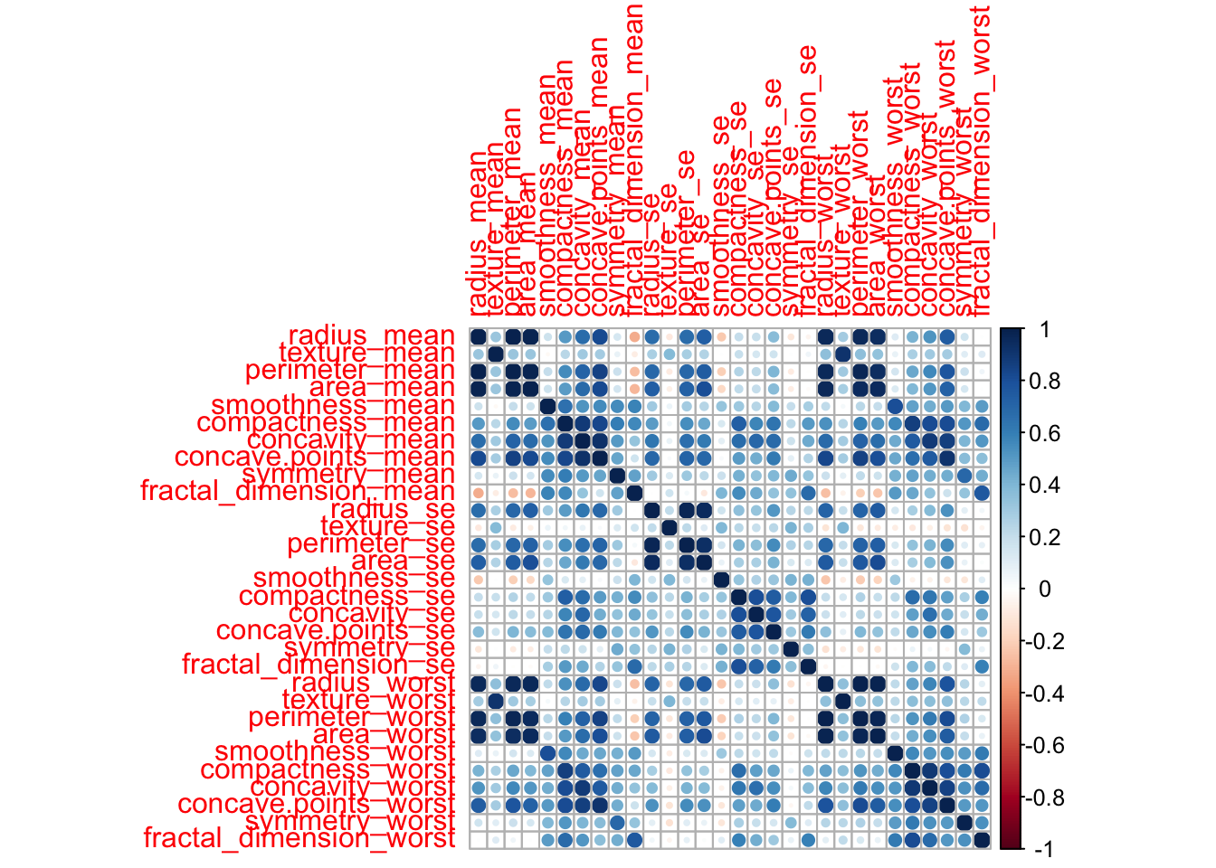
As we can see, some variables, such as radius_mean and perimeter_mean,
have a strong correlation
(r = 0.998).
See the difference in the standard error for radius_mean when it is fitted alone and together with perimeter_mean.
summary(glm(diagnosis == "M" ~ radius_mean ,
            family=binomial,
            data=dados ))
##
## Call:
## glm(formula = diagnosis == "M" ~ radius_mean, family = binomial,
## data = dados)
##
## Deviance Residuals:
## Min 1Q Median 3Q Max
## -2.5470 -0.4694 -0.1746 0.1513 2.8098
##
## Coefficients:
## Estimate Std. Error z value Pr(>|z|)
## (Intercept) -15.24587 1.32463 -11.51 <2e-16 ***
## radius_mean 1.03359 0.09311 11.10 <2e-16 ***
## ---
## Signif. codes: 0 '***' 0.001 '**' 0.01 '*' 0.05 '.' 0.1 ' ' 1
##
## (Dispersion parameter for binomial family taken to be 1)
##
## Null deviance: 751.44 on 568 degrees of freedom
## Residual deviance: 330.01 on 567 degrees of freedom
## AIC: 334.01
##
## Number of Fisher Scoring iterations: 6summary(glm(diagnosis == "M" ~ radius_mean + perimeter_mean,
family=binomial,
data=dados ))##
## Call:
## glm(formula = diagnosis == "M" ~ radius_mean + perimeter_mean,
## family = binomial, data = dados)
##
## Deviance Residuals:
## Min 1Q Median 3Q Max
## -3.0658 -0.3265 -0.1151 0.0942 2.9240
##
## Coefficients:
## Estimate Std. Error z value Pr(>|z|)
## (Intercept) -13.3013 1.4139 -9.408 < 2e-16 ***
## radius_mean -5.7415 0.8995 -6.383 1.74e-10 ***
## perimeter_mean 1.0208 0.1398 7.303 2.82e-13 ***
## ---
## Signif. codes: 0 '***' 0.001 '**' 0.01 '*' 0.05 '.' 0.1 ' ' 1
##
## (Dispersion parameter for binomial family taken to be 1)
##
## Null deviance: 751.44 on 568 degrees of freedom
## Residual deviance: 250.99 on 566 degrees of freedom
## AIC: 256.99
##
## Number of Fisher Scoring iterations: 7The standard error increased almost ten fold. This is due to collinearity and in more extreme cases, there will numeric problems in the maximisation of the likelihood.
For example, if we try to fit a logistic regression with all predictors, we get a message indicating the fitting algorithm did not converge.
summary(glm(diagnosis == "M" ~ .,        #the dot includes all the variables
            family=binomial,
            data=dados[,-1] ))           #remove ID from the dataset
## Warning: glm.fit: algorithm did not converge## Warning: glm.fit: fitted probabilities numerically 0 or 1 occurred##
## Call:
## glm(formula = diagnosis == "M" ~ ., family = binomial, data = dados[,
## -1])
##
## Deviance Residuals:
## Min 1Q Median 3Q Max
## -8.49 -8.49 -8.49 8.49 8.49
##
## Coefficients:
## Estimate Std. Error z value Pr(>|z|)
## (Intercept) -2.881e+06 2.816e+05 -10.233 < 2e-16 ***
## radius_mean 2.427e+06 2.693e+05 9.014 < 2e-16 ***
## texture_mean 1.958e+05 1.471e+04 13.313 < 2e-16 ***
## perimeter_mean 1.473e+06 2.464e+04 59.791 < 2e-16 ***
## area_mean -1.301e+05 3.907e+03 -33.301 < 2e-16 ***
## smoothness_mean -1.525e+08 8.361e+06 -18.234 < 2e-16 ***
## compactness_mean -6.428e+06 3.213e+06 -2.001 0.04539 *
## concavity_mean 1.042e+06 1.408e+06 0.740 0.45959
## concave.points_mean -1.716e+07 5.382e+06 -3.188 0.00143 **
## symmetry_mean 4.049e+07 7.772e+05 52.093 < 2e-16 ***
## fractal_dimension_mean -4.233e+07 2.169e+06 -19.519 < 2e-16 ***
## radius_se 3.328e+07 1.169e+06 28.478 < 2e-16 ***
## texture_se 6.368e+06 2.005e+05 31.763 < 2e-16 ***
## perimeter_se 1.701e+06 4.720e+04 36.032 < 2e-16 ***
## area_se -6.393e+05 1.835e+04 -34.840 < 2e-16 ***
## smoothness_se 7.492e+08 1.224e+07 61.213 < 2e-16 ***
## compactness_se -1.773e+08 5.732e+06 -30.931 < 2e-16 ***
## concavity_se 1.529e+08 5.340e+06 28.624 < 2e-16 ***
## concave.points_se -1.260e+09 4.012e+07 -31.398 < 2e-16 ***
## symmetry_se 2.890e+08 4.126e+06 70.055 < 2e-16 ***
## fractal_dimension_se 1.512e+09 6.597e+07 22.921 < 2e-16 ***
## radius_worst -6.130e+06 2.143e+05 -28.606 < 2e-16 ***
## texture_worst -5.832e+05 2.437e+04 -23.935 < 2e-16 ***
## perimeter_worst -3.538e+05 1.219e+04 -29.023 < 2e-16 ***
## area_worst 8.950e+04 2.741e+03 32.658 < 2e-16 ***
## smoothness_worst -2.161e+07 3.298e+06 -6.553 5.65e-11 ***
## compactness_worst 8.986e+06 3.999e+05 22.470 < 2e-16 ***
## concavity_worst -3.028e+07 1.523e+06 -19.876 < 2e-16 ***
## concave.points_worst 1.431e+08 5.471e+06 26.162 < 2e-16 ***
## symmetry_worst -2.474e+07 3.392e+05 -72.923 < 2e-16 ***
## fractal_dimension_worst -3.698e+07 5.340e+06 -6.926 4.32e-12 ***
## ---
## Signif. codes: 0 '***' 0.001 '**' 0.01 '*' 0.05 '.' 0.1 ' ' 1
##
## (Dispersion parameter for binomial family taken to be 1)
##
## Null deviance: 751.44 on 568 degrees of freedom
## Residual deviance: 32006.76 on 538 degrees of freedom
## AIC: 32069
##
## Number of Fisher Scoring iterations: 25Even if using all the predictors sounds unreasonable, you could think that this would be the first step in using a selection method such as backward stepwise.
Let’s then use lasso to fit the logistic regression. First we need to setup the data:
  X <-  model.matrix(diagnosis ~  .,
                     data=dados[,-1])[,-1]  #dados[,-1] exclude the ID var
                                            #the other [,-1] excludes the
                                            #column of 1's from the design
                                            #matrix
  #X <-  as.matrix(dados[,-c(1,2)])         #this would be another way of
                                            #defining X
  Y <- dados[,"diagnosis"]=="M"             #makes the outcome binary
Now we can find \(\lambda\) by cross-validation.
  cv.model<- cv.glmnet(x=X,y=Y,
                       family = "binomial",
                       alpha=1)                        #alpha=1 is lasso

  plot(cv.model)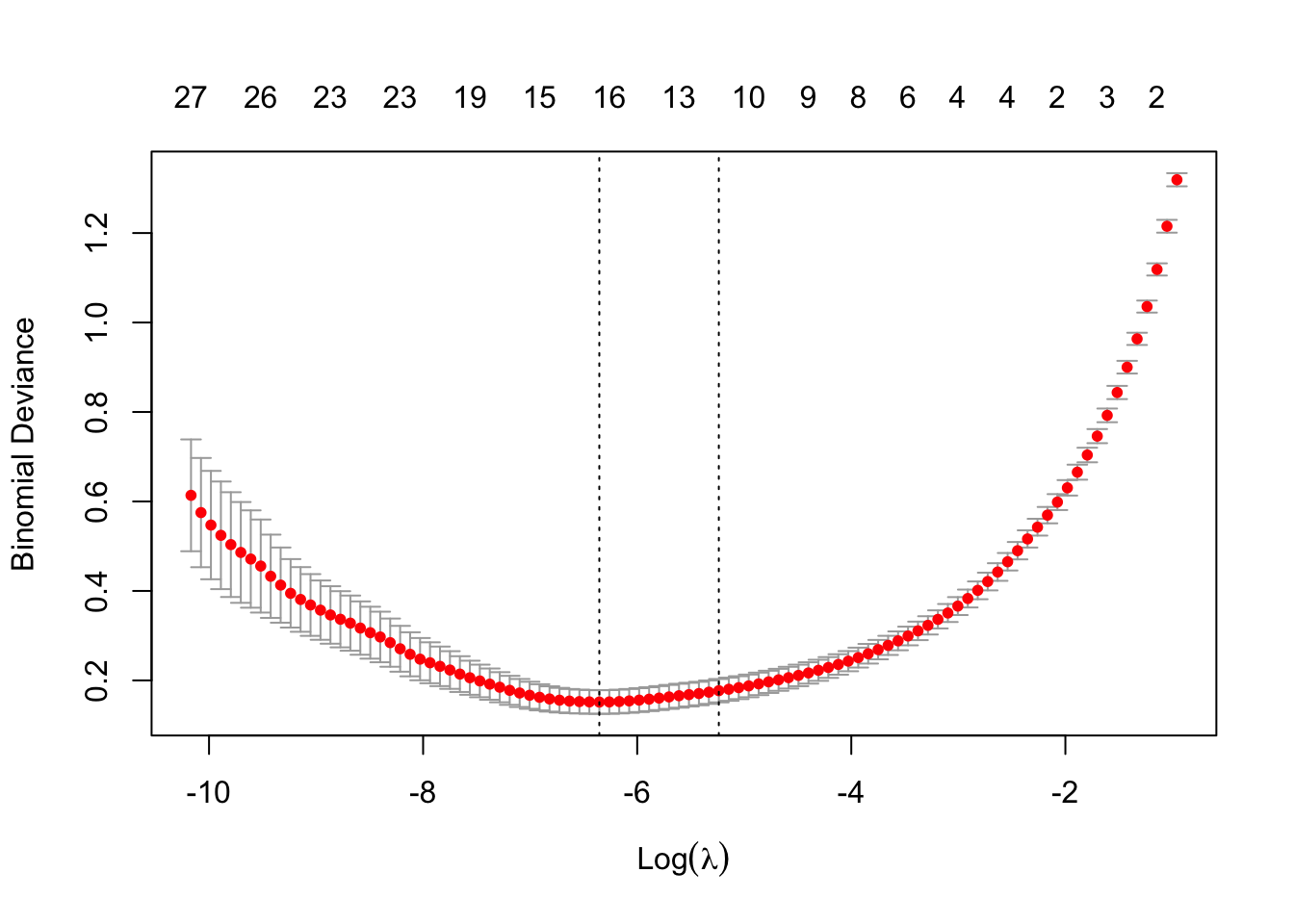
l.min <- cv.model$lambda.minNOTE: Notice that for the logistic regression we do not use the mean squared error as the loss function. Instead, we can use another loss function, such as the exponential loss of the binomial deviance loss. You can see in the plot showing the cross-validation results for \(\lambda\), that the y-axis is the binomial deviance.
We can now use use the \(\lambda\) with minimum deviance (\(\lambda = exp(-6.35)\)) to fit the final lasso logistic model
lasso.model <- glmnet(x=X,y=Y,
                      family = "binomial",
                      alpha=1,
                      lambda = l.min)

lasso.model$beta
## 30 x 1 sparse Matrix of class "dgCMatrix"
## s0
## radius_mean .
## texture_mean .
## perimeter_mean .
## area_mean .
## smoothness_mean .
## compactness_mean .
## concavity_mean 1.057681617
## concave.points_mean 28.653197982
## symmetry_mean .
## fractal_dimension_mean -19.641695432
## radius_se 9.794444752
## texture_se -0.713988108
## perimeter_se .
## area_se .
## smoothness_se 107.757070444
## compactness_se -48.930433022
## concavity_se .
## concave.points_se .
## symmetry_se .
## fractal_dimension_se -89.643202541
## radius_worst 0.393454819
## texture_worst 0.290988915
## perimeter_worst 0.004763114
## area_worst 0.004211633
## smoothness_worst 23.687603116
## compactness_worst .
## concavity_worst 5.415615601
## concave.points_worst 19.301146713
## symmetry_worst 8.936536781
## fractal_dimension_worst .And we can evaluate the logistic model using the methods that we have seen
before. The function assess.glmnet() gives several statistics, including the
area under the ROC curve (c-statistics). The roc.glmnet() produces the
coordinates for the ROC curve
assess.glmnet(lasso.model,           #in this case, we are evaluating the model
              newx = X,              #in the same data used to fit the model
              newy = Y )             #so newx=X and newY=Y
## $deviance
## s0
## 0.1071175
## attr(,"measure")
## [1] "Binomial Deviance"
##
## $class
## s0
## 0.01054482
## attr(,"measure")
## [1] "Misclassification Error"
##
## $auc
## [1] 0.9977406
## attr(,"measure")
## [1] "AUC"
##
## $mse
## s0
## 0.02640251
## attr(,"measure")
## [1] "Mean-Squared Error"
##
## $mae
## s0
## 0.07270511
## attr(,"measure")
## [1] "Mean Absolute Error"plot(roc.glmnet(lasso.model,
newx = X,
newy = Y ),
type="l") #produces the ROC plot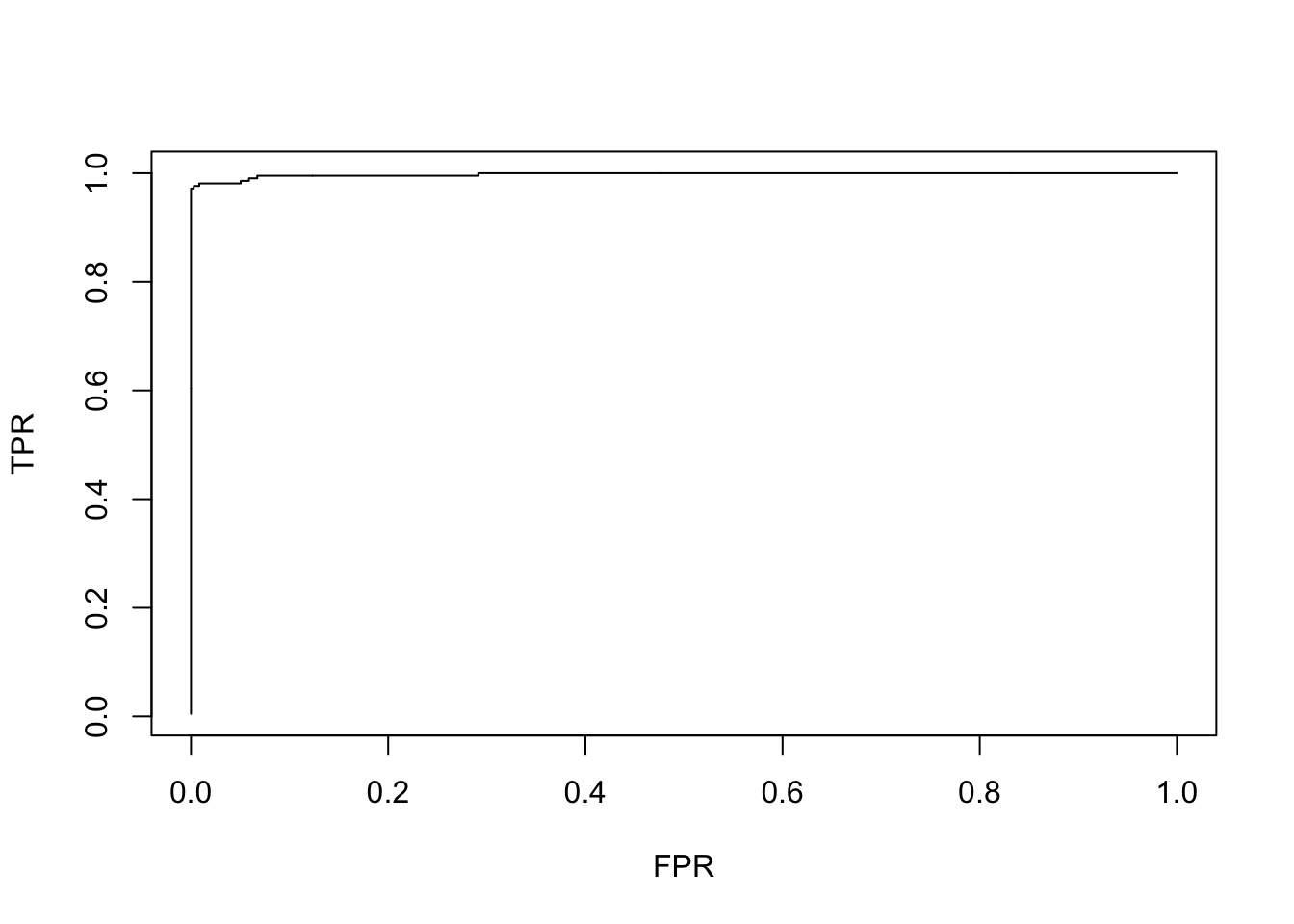
Notice, that the model can almost predict the outcome, at least in the same data used to fit the model.
TRY IT YOURSELF:
- Produce the lasso path for the estimates
See the solution code
plot(cv.model$glmnet.fit, xvar="lambda")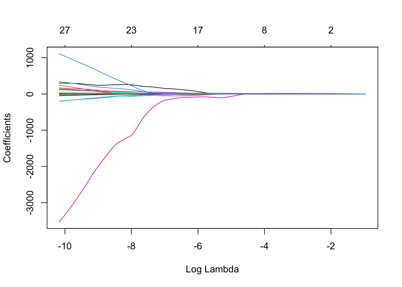
4.4 Exercises
Solve the following exercise:
The dataset fat is available in the library(faraway). The data set contains several physical measurements.
Fit a linear model to predict body fat (variable brozek) using all other predictors except for siri, density and free. Get the lasso estimates and compare them with the OLS and ridge estimates.
The dataset
prostateavailable in the packagefarawaycontains information on 97 men who were about to receive a radical prostatectomy. These data come from a study examining the correlation between the prostate specific antigen (logpsa) and a number of other clinical measures.Use lasso to fit the linear model and compare the variables selected with the a backward stepwise to predict logpsa using all other predictors.