1 Best Subset Selection
1.1 Introduction
Suppose that we have available a set of variables to predict an outcome of interest and want to choose a subset of those variable that accurately predict the outcome.
Once we have decided of the type of model (logistic regression, for example), one option is to fit all the possible combination of variables and choose the one with best criteria according to some criteria. This is called best subset selection.
This approach is computationally demanding. With \(p\) potential predictors, we need to fit \(2^p\) models. Additionally, if we want to use cross-validation to evaluate their performance, the problem quickly becomes unfeasible.The leaps and bounds algorithm speeds up the search of the “best” models and it does not require fitting all the models. In any case, even this algorithm does not help if the number of predictors is to large.
The leaps and bounds algorithm is implemented in the `leaps package. If
you want to know more about the leaps and bounds approach you can read the
original article by Furnival and Wilson
but this is behyond the contents of this unit.
1.3 Practical session
Task 1 - Fit the best subset linear model
With the fat dataset in the library(faraway), we want to fit a linear model to predict body fat (variable brozek) using the other variables available, except for siri (another way of computing body fat), density (it is used in the brozek and siri formulas) and free (it is computed using brozek formula)
Let’s first read the data
#install.packages(c("leaps", "faraway"))
library(leaps)   #function to search for the best model
library(faraway) #has the dataset fat
set.seed(1212)data("fat")
head(fat)## brozek siri density age weight height adipos free neck chest abdom hip
## 1 12.6 12.3 1.0708 23 154.25 67.75 23.7 134.9 36.2 93.1 85.2 94.5
## 2 6.9 6.1 1.0853 22 173.25 72.25 23.4 161.3 38.5 93.6 83.0 98.7
## 3 24.6 25.3 1.0414 22 154.00 66.25 24.7 116.0 34.0 95.8 87.9 99.2
## 4 10.9 10.4 1.0751 26 184.75 72.25 24.9 164.7 37.4 101.8 86.4 101.2
## 5 27.8 28.7 1.0340 24 184.25 71.25 25.6 133.1 34.4 97.3 100.0 101.9
## 6 20.6 20.9 1.0502 24 210.25 74.75 26.5 167.0 39.0 104.5 94.4 107.8
## thigh knee ankle biceps forearm wrist
## 1 59.0 37.3 21.9 32.0 27.4 17.1
## 2 58.7 37.3 23.4 30.5 28.9 18.2
## 3 59.6 38.9 24.0 28.8 25.2 16.6
## 4 60.1 37.3 22.8 32.4 29.4 18.2
## 5 63.2 42.2 24.0 32.2 27.7 17.7
## 6 66.0 42.0 25.6 35.7 30.6 18.8The function regsubsets() will produce the best model with 1 predictor, the best model with 2 predictors, 3 predictors, … up to 14 predictors(nvmax=14 option).
##############################################################################
#Best subset model
##############################################################################
bestsub.model <- regsubsets(brozek ~ age +
                              weight + height +
                              adipos +
                              neck + chest +
                              abdom + hip +
                              thigh + knee +
                              ankle +biceps +
                              forearm + wrist,
                            data = fat, nvmax = 14)

summary(bestsub.model)
## Subset selection object
## Call: regsubsets.formula(brozek ~ age + weight + height + adipos +
## neck + chest + abdom + hip + thigh + knee + ankle + biceps +
## forearm + wrist, data = fat, nvmax = 14)
## 14 Variables (and intercept)
## Forced in Forced out
## age FALSE FALSE
## weight FALSE FALSE
## height FALSE FALSE
## adipos FALSE FALSE
## neck FALSE FALSE
## chest FALSE FALSE
## abdom FALSE FALSE
## hip FALSE FALSE
## thigh FALSE FALSE
## knee FALSE FALSE
## ankle FALSE FALSE
## biceps FALSE FALSE
## forearm FALSE FALSE
## wrist FALSE FALSE
## 1 subsets of each size up to 14
## Selection Algorithm: exhaustive
## age weight height adipos neck chest abdom hip thigh knee ankle biceps
## 1 ( 1 ) " " " " " " " " " " " " "*" " " " " " " " " " "
## 2 ( 1 ) " " "*" " " " " " " " " "*" " " " " " " " " " "
## 3 ( 1 ) " " "*" " " " " " " " " "*" " " " " " " " " " "
## 4 ( 1 ) " " "*" " " " " " " " " "*" " " " " " " " " " "
## 5 ( 1 ) " " "*" " " " " "*" " " "*" " " " " " " " " " "
## 6 ( 1 ) "*" "*" " " " " " " " " "*" " " "*" " " " " " "
## 7 ( 1 ) "*" "*" " " " " "*" " " "*" " " "*" " " " " " "
## 8 ( 1 ) "*" "*" " " " " "*" " " "*" "*" "*" " " " " " "
## 9 ( 1 ) "*" "*" " " " " "*" " " "*" "*" "*" " " " " "*"
## 10 ( 1 ) "*" "*" " " " " "*" " " "*" "*" "*" " " "*" "*"
## 11 ( 1 ) "*" "*" "*" " " "*" " " "*" "*" "*" " " "*" "*"
## 12 ( 1 ) "*" "*" "*" " " "*" "*" "*" "*" "*" " " "*" "*"
## 13 ( 1 ) "*" "*" "*" "*" "*" "*" "*" "*" "*" " " "*" "*"
## 14 ( 1 ) "*" "*" "*" "*" "*" "*" "*" "*" "*" "*" "*" "*"
## forearm wrist
## 1 ( 1 ) " " " "
## 2 ( 1 ) " " " "
## 3 ( 1 ) " " "*"
## 4 ( 1 ) "*" "*"
## 5 ( 1 ) "*" "*"
## 6 ( 1 ) "*" "*"
## 7 ( 1 ) "*" "*"
## 8 ( 1 ) "*" "*"
## 9 ( 1 ) "*" "*"
## 10 ( 1 ) "*" "*"
## 11 ( 1 ) "*" "*"
## 12 ( 1 ) "*" "*"
## 13 ( 1 ) "*" "*"
## 14 ( 1 ) "*" "*"In the result above, we can see that the best model with 1 predictor has the variable abdom, the best with 2 predictors has weight and free, and the last one has all the 15 variables.
Notice that these models were not chosen with cross-validation. Within the models with the same number of predictors, the model with higher \(r^2\) is chosen (however, I could not find in the leaps() documentation that this is, in fact, the criteria).
We can then use other statistics such as \(Cp\), \(adjusted-r^2\) or \(BIC\) to choose among the selected 17 models
#Performance measures
  cbind(
    Cp     = summary(bestsub.model)$cp,
    r2     = summary(bestsub.model)$rsq,
    Adj_r2 = summary(bestsub.model)$adjr2,
    BIC    =summary(bestsub.model)$bic
)
## Cp r2 Adj_r2 BIC
## [1,] 71.075501 0.6621178 0.6607663 -262.3758
## [2,] 19.617727 0.7187265 0.7164672 -303.0555
## [3,] 13.279341 0.7275563 0.7242606 -305.5638
## [4,] 8.147986 0.7351080 0.7308182 -307.1180
## [5,] 7.412297 0.7380049 0.7326798 -304.3597
## [6,] 6.590118 0.7409935 0.7346504 -301.7213
## [7,] 5.311670 0.7444651 0.7371342 -299.5925
## [8,] 5.230664 0.7466688 0.7383287 -296.2456
## [9,] 6.296894 0.7476576 0.7382730 -291.7018
## [10,] 7.595324 0.7484005 0.7379607 -286.9153
## [11,] 9.114827 0.7489093 0.7374010 -281.8960
## [12,] 11.050872 0.7489771 0.7363734 -276.4346
## [13,] 13.000019 0.7490309 0.7353225 -270.9592
## [14,] 15.000000 0.7490309 0.7342058 -265.4298In this case, depending on the performance statistic used, we could have selected models with 4 variables (according to \(BIC\)) up to 8 variables (\(adjusted-r^2\) ).
Another option is to use cross-validation in this subset of model. Below,
a leave-one-out cross-validation is used to choose the model with lowest \(MSE\).
The function regsubset() does not include a
prediction function. So, we start by programming a function to get predictions
out of regsubset() .
##Function to get predictions from the regsubset function
predict.regsubsets <- function(object, newdata, id,...){
  form  <- as.formula(object$call[[2]])
  mat   <- model.matrix(form, newdata)
  coefi <- coef(object, id=id)
  mat[, names(coefi)]%*%coefi
}
We know implement the leave-one-out cross-validation by regsubset() in
\(n-1\) observations and getting the prediction error in the excluded observation.
We repeat this \(n\) times
##jack-knife validation (leave-one-out)

  #store the prediction error n=252
  jk.errors <- matrix(NA, 252, 14)

  for (k in 1:252){
    #uses regsubsets in the data with 1 observation removed
    best.model.cv <- regsubsets(brozek ~ age +
                          weight + height +
                          adipos + neck + chest +
                          abdom + hip + thigh +
                          knee + ankle + biceps +
                          forearm + wrist,
                        data = fat[-k,],          #removes the kth obsv
                        nvmax = 14)

    #Models with 1, 2 ,...14 predictors
    for (i in 1:14){
      #that was left out
      pred <- predict(best.model.cv,                 #prediction in the obsv
                      fat[k,],
                      id=i)
      jk.errors[k,i] <- (fat$brozek[k]-pred)^2       #error in the obsv
    }
  }

  mse.models <- apply(jk.errors, 2, mean)            #MSE estimation
      plot(mse.models ,                              #Plot with MSEs
       pch=19, type="b",
       xlab="nr predictors",
       ylab="MSE")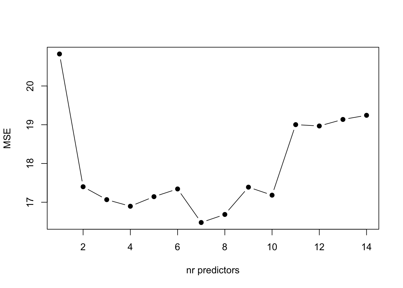
From the plot above, we can see that the model with 7 predictors is the one with lower \(MSE\).
From the initial matrix of models, we can see that the one with 7 predictors include age, weight, weight, neck, abdom, thigh, forearm and wrist. This model is presented below:
#final model from exhaustive search
  final.model <- lm(brozek ~  age +
                      weight + neck +
                      abdom + thigh +
                      forearm + wrist,
                    data = fat)
  summary(final.model)
##
## Call:
## lm(formula = brozek ~ age + weight + neck + abdom + thigh + forearm +
## wrist, data = fat)
##
## Residuals:
## Min 1Q Median 3Q Max
## -10.0193 -2.8016 -0.1234 2.9387 9.0019
##
## Coefficients:
## Estimate Std. Error t value Pr(>|t|)
## (Intercept) -30.17420 8.34200 -3.617 0.000362 ***
## age 0.06149 0.02852 2.156 0.032047 *
## weight -0.11236 0.03151 -3.565 0.000437 ***
## neck -0.37203 0.20434 -1.821 0.069876 .
## abdom 0.85152 0.06437 13.229 < 2e-16 ***
## thigh 0.20973 0.10745 1.952 0.052099 .
## forearm 0.51824 0.17115 3.028 0.002726 **
## wrist -1.40081 0.47274 -2.963 0.003346 **
## ---
## Signif. codes: 0 '***' 0.001 '**' 0.01 '*' 0.05 '.' 0.1 ' ' 1
##
## Residual standard error: 3.974 on 244 degrees of freedom
## Multiple R-squared: 0.7445, Adjusted R-squared: 0.7371
## F-statistic: 101.6 on 7 and 244 DF, p-value: < 2.2e-16TRY IT YOURSELF:
- For the estimation of the MSE above, use 10 repeated 5-fold cross-validation (repeat the 5-fold cv 10 times) instead of leave-one-out.
See the solution code
#####################################################
#1) ALTERNATIVE 10 times 5-fold Cross-validation
#####################################################
  predict.regsubsets <- function(object, newdata, id,...){
    form  <- as.formula(object$call[[2]])
    mat   <- model.matrix(form, newdata)
    coefi <- coef(object, id=id)
    mat[, names(coefi)]%*%coefi
  }

  mse.cv<-matrix(NA, 10, 14)
  for (j in 1:10){                            #repeat cv 10 times
    k.fold <- 5
    folds <- sample(rep(1:k.fold,             #Assigns each observation to a fold
                        length=nrow(fat)))

    cv.errors <- matrix(NA, k.fold, 14)       #store the errors

    for (k in 1:k.fold){
      best.model.cv <-  regsubsets(brozek ~ age +
                                     weight + height +
                                     adipos +
                                     neck + chest +
                                     abdom + hip +
                                     thigh + knee +
                                     ankle + biceps +
                                     forearm + wrist,
                                   data = fat[folds!=k,],   #uses all but
                                   nvmax = 14)              #the k-fold
      for (i in 1:14){
        pred <- predict(best.model.cv,
                        fat[folds==k,], id=i)               #predict the k-fold
        cv.errors[k,i] = mean((fat$brozek[folds==k]-pred)^2)
      }
    }
    mse.cv[j,]=apply(cv.errors, 2, mean)
  }

  plot(apply(mse.cv, 2, mean), pch=19, type="b")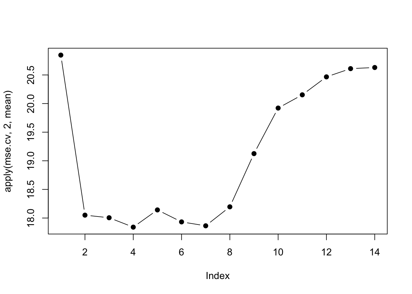
############################################################Task 2 - Fit the best subset logistic model
With the lowbwt.csv dataset, in the library(faraway), we want to fit a logistic regression to predict low birthweight (<2500gr), using age, lwt, race ,smoke, ptl, ht, ui, ftv.
Let’s read the data and make sure that race and ftv are factor predictors. And recode ftv into (0, 1, 2+)
#install.packages("bestglm")
#install.packages("dplyr")
library(bestglm)
library(dplyr)                            #to use the rename() function
##
## Attaching package: 'dplyr'## The following objects are masked from 'package:stats':
##
## filter, lag## The following objects are masked from 'package:base':
##
## intersect, setdiff, setequal, unionlowbwt <- read.csv("https://www.dropbox.com/s/1odxxsbwd5anjs8/lowbwt.csv?dl=1",
stringsAsFactors = TRUE)
lowbwt$race <- factor(lowbwt$race,
levels = c(1,2,3),
labels = c("White", "Black", "Other"))
#number of previous appointments
lowbwt$ftv[lowbwt$ftv>1] <- 2 #categories 0, 1, 2+
lowbwt$ftv <- factor(lowbwt$ftv,
levels = c(0,1,2),
labels = c("0", "1", "2+"))
head(lowbwt)## id low age lwt race smoke ptl ht ui ftv bwt
## 1 85 0 19 182 Black 0 0 0 1 0 2523
## 2 86 0 33 155 Other 0 0 0 0 2+ 2551
## 3 87 0 20 105 White 1 0 0 0 1 2557
## 4 88 0 21 108 White 1 0 0 1 2+ 2594
## 5 89 0 18 107 White 1 0 0 1 0 2600
## 6 91 0 21 124 Other 0 0 0 0 0 2622The regsubets() function only fits linear model. The package bestglm
fits generalised linear models.
The syntax for the function bestglm() is different from other functions.
The data need to be in the format Xy, where X are the predictors and
the last variable in the dataset is the outcome that needs to be labeled y.
lowbwt.bglm <- lowbwt[, c("age", "lwt", "race",
                              "smoke", "ptl",
                              "ht", "ui", "ftv", "low")]
rename(lowbwt.bglm, y=low)
## age lwt race smoke ptl ht ui ftv y
## 1 19 182 Black 0 0 0 1 0 0
## 2 33 155 Other 0 0 0 0 2+ 0
## 3 20 105 White 1 0 0 0 1 0
## 4 21 108 White 1 0 0 1 2+ 0
## 5 18 107 White 1 0 0 1 0 0
## 6 21 124 Other 0 0 0 0 0 0
## 7 22 118 White 0 0 0 0 1 0
## 8 17 103 Other 0 0 0 0 1 0
## 9 29 123 White 1 0 0 0 1 0
## 10 26 113 White 1 0 0 0 0 0
## 11 19 95 Other 0 0 0 0 0 0
## 12 19 150 Other 0 0 0 0 1 0
## 13 22 95 Other 0 0 1 0 0 0
## 14 30 107 Other 0 1 0 1 2+ 0
## 15 18 100 White 1 0 0 0 0 0
## 16 18 100 White 1 0 0 0 0 0
## 17 15 98 Black 0 0 0 0 0 0
## 18 25 118 White 1 0 0 0 2+ 0
## 19 20 120 Other 0 0 0 1 0 0
## 20 28 120 White 1 0 0 0 1 0
## 21 32 121 Other 0 0 0 0 2+ 0
## 22 31 100 White 0 0 0 1 2+ 0
## 23 36 202 White 0 0 0 0 1 0
## 24 28 120 Other 0 0 0 0 0 0
## 25 25 120 Other 0 0 0 1 2+ 0
## 26 28 167 White 0 0 0 0 0 0
## 27 17 122 White 1 0 0 0 0 0
## 28 29 150 White 0 0 0 0 2+ 0
## 29 26 168 Black 1 0 0 0 0 0
## 30 17 113 Black 0 0 0 0 1 0
## 31 17 113 Black 0 0 0 0 1 0
## 32 24 90 White 1 1 0 0 1 0
## 33 35 121 Black 1 1 0 0 1 0
## 34 25 155 White 0 0 0 0 1 0
## 35 25 125 Black 0 0 0 0 0 0
## 36 29 140 White 1 0 0 0 2+ 0
## 37 19 138 White 1 0 0 0 2+ 0
## 38 27 124 White 1 0 0 0 0 0
## 39 31 215 White 1 0 0 0 2+ 0
## 40 33 109 White 1 0 0 0 1 0
## 41 21 185 Black 1 0 0 0 2+ 0
## 42 19 189 White 0 0 0 0 2+ 0
## 43 23 130 Black 0 0 0 0 1 0
## 44 21 160 White 0 0 0 0 0 0
## 45 18 90 White 1 0 0 1 0 0
## 46 18 90 White 1 0 0 1 0 0
## 47 32 132 White 0 0 0 0 2+ 0
## 48 19 132 Other 0 0 0 0 0 0
## 49 24 115 White 0 0 0 0 2+ 0
## 50 22 85 Other 1 0 0 0 0 0
## 51 22 120 White 0 0 1 0 1 0
## 52 23 128 Other 0 0 0 0 0 0
## 53 22 130 White 1 0 0 0 0 0
## 54 30 95 White 1 0 0 0 2+ 0
## 55 19 115 Other 0 0 0 0 0 0
## 56 16 110 Other 0 0 0 0 0 0
## 57 21 110 Other 1 0 0 1 0 0
## 58 30 153 Other 0 0 0 0 0 0
## 59 20 103 Other 0 0 0 0 0 0
## 60 17 119 Other 0 0 0 0 0 0
## 61 17 119 Other 0 0 0 0 0 0
## 62 23 119 Other 0 0 0 0 2+ 0
## 63 24 110 Other 0 0 0 0 0 0
## 64 28 140 White 0 0 0 0 0 0
## 65 26 133 Other 1 2 0 0 0 0
## 66 20 169 Other 0 1 0 1 1 0
## 67 24 115 Other 0 0 0 0 2+ 0
## 68 28 250 Other 1 0 0 0 2+ 0
## 69 20 141 White 0 2 0 1 1 0
## 70 22 158 Black 0 1 0 0 2+ 0
## 71 22 112 White 1 2 0 0 0 0
## 72 31 150 Other 1 0 0 0 2+ 0
## 73 23 115 Other 1 0 0 0 1 0
## 74 16 112 Black 0 0 0 0 0 0
## 75 16 135 White 1 0 0 0 0 0
## 76 18 229 Black 0 0 0 0 0 0
## 77 25 140 White 0 0 0 0 1 0
## 78 32 134 White 1 1 0 0 2+ 0
## 79 20 121 Black 1 0 0 0 0 0
## 80 23 190 White 0 0 0 0 0 0
## 81 22 131 White 0 0 0 0 1 0
## 82 32 170 White 0 0 0 0 0 0
## 83 30 110 Other 0 0 0 0 0 0
## 84 20 127 Other 0 0 0 0 0 0
## 85 23 123 Other 0 0 0 0 0 0
## 86 17 120 Other 1 0 0 0 0 0
## 87 19 105 Other 0 0 0 0 0 0
## 88 23 130 White 0 0 0 0 0 0
## 89 36 175 White 0 0 0 0 0 0
## 90 22 125 White 0 0 0 0 1 0
## 91 24 133 White 0 0 0 0 0 0
## 92 21 134 Other 0 0 0 0 2+ 0
## 93 19 235 White 1 0 1 0 0 0
## 94 25 95 White 1 3 0 1 0 0
## 95 16 135 White 1 0 0 0 0 0
## 96 29 135 White 0 0 0 0 1 0
## 97 29 154 White 0 0 0 0 1 0
## 98 19 147 White 1 0 0 0 0 0
## 99 19 147 White 1 0 0 0 0 0
## 100 30 137 White 0 0 0 0 1 0
## 101 24 110 White 0 0 0 0 1 0
## 102 19 184 White 1 0 1 0 0 0
## 103 24 110 Other 0 1 0 0 0 0
## 104 23 110 White 0 0 0 0 1 0
## 105 20 120 Other 0 0 0 0 0 0
## 106 25 241 Black 0 0 1 0 0 0
## 107 30 112 White 0 0 0 0 1 0
## 108 22 169 White 0 0 0 0 0 0
## 109 18 120 White 1 0 0 0 2+ 0
## 110 16 170 Black 0 0 0 0 2+ 0
## 111 32 186 White 0 0 0 0 2+ 0
## 112 18 120 Other 0 0 0 0 1 0
## 113 29 130 White 1 0 0 0 2+ 0
## 114 33 117 White 0 0 0 1 1 0
## 115 20 170 White 1 0 0 0 0 0
## 116 28 134 Other 0 0 0 0 1 0
## 117 14 135 White 0 0 0 0 0 0
## 118 28 130 Other 0 0 0 0 0 0
## 119 25 120 White 0 0 0 0 2+ 0
## 120 16 95 Other 0 0 0 0 1 0
## 121 20 158 White 0 0 0 0 1 0
## 122 26 160 Other 0 0 0 0 0 0
## 123 21 115 White 0 0 0 0 1 0
## 124 22 129 White 0 0 0 0 0 0
## 125 25 130 White 0 0 0 0 2+ 0
## 126 31 120 White 0 0 0 0 2+ 0
## 127 35 170 White 0 1 0 0 1 0
## 128 19 120 White 1 0 0 0 0 0
## 129 24 116 White 0 0 0 0 1 0
## 130 45 123 White 0 0 0 0 1 0
## 131 28 120 Other 1 1 0 1 0 1
## 132 29 130 White 0 0 0 1 2+ 1
## 133 34 187 Black 1 0 1 0 0 1
## 134 25 105 Other 0 1 1 0 0 1
## 135 25 85 Other 0 0 0 1 0 1
## 136 27 150 Other 0 0 0 0 0 1
## 137 23 97 Other 0 0 0 1 1 1
## 138 24 128 Black 0 1 0 0 1 1
## 139 24 132 Other 0 0 1 0 0 1
## 140 21 165 White 1 0 1 0 1 1
## 141 32 105 White 1 0 0 0 0 1
## 142 19 91 White 1 2 0 1 0 1
## 143 25 115 Other 0 0 0 0 0 1
## 144 16 130 Other 0 0 0 0 1 1
## 145 25 92 White 1 0 0 0 0 1
## 146 20 150 White 1 0 0 0 2+ 1
## 147 21 200 Black 0 0 0 1 2+ 1
## 148 24 155 White 1 1 0 0 0 1
## 149 21 103 Other 0 0 0 0 0 1
## 150 20 125 Other 0 0 0 1 0 1
## 151 25 89 Other 0 2 0 0 1 1
## 152 19 102 White 0 0 0 0 2+ 1
## 153 19 112 White 1 0 0 1 0 1
## 154 26 117 White 1 1 0 0 0 1
## 155 24 138 White 0 0 0 0 0 1
## 156 17 130 Other 1 1 0 1 0 1
## 157 20 120 Black 1 0 0 0 2+ 1
## 158 22 130 White 1 1 0 1 1 1
## 159 27 130 Black 0 0 0 1 0 1
## 160 20 80 Other 1 0 0 1 0 1
## 161 17 110 White 1 0 0 0 0 1
## 162 25 105 Other 0 1 0 0 1 1
## 163 20 109 Other 0 0 0 0 0 1
## 164 18 148 Other 0 0 0 0 0 1
## 165 18 110 Black 1 1 0 0 0 1
## 166 20 121 White 1 1 0 1 0 1
## 167 21 100 Other 0 1 0 0 2+ 1
## 168 26 96 Other 0 0 0 0 0 1
## 169 31 102 White 1 1 0 0 1 1
## 170 15 110 White 0 0 0 0 0 1
## 171 23 187 Black 1 0 0 0 1 1
## 172 20 122 Black 1 0 0 0 0 1
## 173 24 105 Black 1 0 0 0 0 1
## 174 15 115 Other 0 0 0 1 0 1
## 175 23 120 Other 0 0 0 0 0 1
## 176 30 142 White 1 1 0 0 0 1
## 177 22 130 White 1 0 0 0 1 1
## 178 17 120 White 1 0 0 0 2+ 1
## 179 23 110 White 1 1 0 0 0 1
## 180 17 120 Black 0 0 0 0 2+ 1
## 181 26 154 Other 0 1 1 0 1 1
## 182 20 105 Other 0 0 0 0 2+ 1
## 183 26 190 White 1 0 0 0 0 1
## 184 14 101 Other 1 1 0 0 0 1
## 185 28 95 White 1 0 0 0 2+ 1
## 186 14 100 Other 0 0 0 0 2+ 1
## 187 23 94 Other 1 0 0 0 0 1
## 188 17 142 Black 0 0 1 0 0 1
## 189 21 130 White 1 0 1 0 2+ 1And new we choose among all the models with combinations of the predictors using the \(AIC\) criteria (or any other)
best.logit <- bestglm(lowbwt.bglm,
                IC = "AIC",                 # Information criteria for
                family=binomial,
                method = "exhaustive")
## Morgan-Tatar search since family is non-gaussian.## Note: factors present with more than 2 levels.summary(best.logit$BestModel)##
## Call:
## glm(formula = y ~ ., family = family, data = Xi, weights = weights)
##
## Deviance Residuals:
## Min 1Q Median 3Q Max
## -1.9049 -0.8124 -0.5241 0.9483 2.1812
##
## Coefficients:
## Estimate Std. Error z value Pr(>|z|)
## (Intercept) -0.086550 0.951760 -0.091 0.92754
## lwt -0.015905 0.006855 -2.320 0.02033 *
## raceBlack 1.325719 0.522243 2.539 0.01113 *
## raceOther 0.897078 0.433881 2.068 0.03868 *
## smoke 0.938727 0.398717 2.354 0.01855 *
## ptl 0.503215 0.341231 1.475 0.14029
## ht 1.855042 0.695118 2.669 0.00762 **
## ui 0.785698 0.456441 1.721 0.08519 .
## ---
## Signif. codes: 0 '***' 0.001 '**' 0.01 '*' 0.05 '.' 0.1 ' ' 1
##
## (Dispersion parameter for binomial family taken to be 1)
##
## Null deviance: 234.67 on 188 degrees of freedom
## Residual deviance: 201.99 on 181 degrees of freedom
## AIC: 217.99
##
## Number of Fisher Scoring iterations: 4Repeating the same exercise as we have done with the linear model, where we have cross-validated all the best models with 1, 2, …., 8 predictors, is also possible. The variables selected for each one of those best models are:
best.logit$Subsets## Intercept age lwt race smoke ptl ht ui ftv logLikelihood
## 0 TRUE FALSE FALSE FALSE FALSE FALSE FALSE FALSE FALSE -117.3360
## 1 TRUE FALSE FALSE FALSE FALSE TRUE FALSE FALSE FALSE -113.9463
## 2 TRUE FALSE TRUE FALSE FALSE FALSE TRUE FALSE FALSE -110.5710
## 3 TRUE FALSE TRUE FALSE FALSE TRUE TRUE FALSE FALSE -107.9819
## 4 TRUE FALSE TRUE TRUE TRUE FALSE TRUE FALSE FALSE -104.1237
## 5 TRUE FALSE TRUE TRUE TRUE FALSE TRUE TRUE FALSE -102.1083
## 6* TRUE FALSE TRUE TRUE TRUE TRUE TRUE TRUE FALSE -100.9928
## 7 TRUE TRUE TRUE TRUE TRUE TRUE TRUE TRUE FALSE -100.7135
## 8 TRUE TRUE TRUE TRUE TRUE TRUE TRUE TRUE TRUE -100.3030
## AIC
## 0 234.6720
## 1 229.8926
## 2 225.1421
## 3 221.9638
## 4 218.2474
## 5 216.2166
## 6* 215.9856
## 7 217.4270
## 8 220.6061We could now run a cross validation for each one of those models and compute the area under the ROC as measure of performance.
1.4 Exercises
Solve the following exercise:
The dataset fat is available in the library(faraway). The data set contains several physical measurements.
Select the best subset model to predict body fat (variable brozek) using all other predictors except for siri, density and free. You can use the \(adjusted-r^2\) to select the best model
The dataset
prostateavailable in the packagefarawaycontains information on 97 men who were about to receive a radical prostatectomy. These data come from a study examining the correlation between the prostate specific antigen (logpsa) and a number of other clinical measures.Select the best subset model to predict logpsa using all other predictors. You can use the \(adjusted-r^2\) to select the best model