9 Probability and Inference

9.1 Probability:

Probability is a numerical measure of the likelihood that a particular event will occur. It ranges from 0 to 1, with 0 meaning the event is impossible and 1 meaning the event is certain. Probabilities can be represented graphically using bar plots or pie charts.

9.2 Sample Space:

The sample space is the set of all possible outcomes for a given experiment or event. For example, in a coin toss experiment, the sample space is {Heads, Tails}. The sample space can be represented using Venn diagrams or tree diagrams.

9.3 Conditional Probability:

Conditional probability refers to the probability of an event occurring given that another event has already occurred. It can be represented graphically using Venn diagrams, which show the intersections of events.

9.4 Independence:

Two events are independent if the occurrence of one event does not affect the probability of the other event. Graphically, independence can be visualized using Venn diagrams or probability tables, where the probability of the intersection of two events is equal to the product of their individual probabilities.

9.5 Bayes’ Theorem:

Bayes’ theorem is a powerful tool for updating the probability of an event based on new evidence. It can be visualized using tree diagrams or probability tables, which show the updated probabilities after taking into account the new evidence.

9.6 Discrete and Continuous Probability Distributions:

Discrete probability distributions describe the probabilities of outcomes for discrete random variables (e.g., number of heads in coin tosses), while continuous probability distributions describe the probabilities of outcomes for continuous random variables (e.g., height of individuals). Discrete distributions can be visualized using bar plots, and continuous distributions can be visualized using probability density functions or cumulative distribution functions.

#Sampling distribution

A sampling distribution is the probability distribution of a sample statistic (e.g., sample mean, sample proportion) obtained from a population. It helps to understand the variability of the sample statistic and the likelihood of obtaining different sample statistics from the population.

9.7 Central Limit Theorem

The CLT states that, for a large enough sample size (usually n ≥ 30), the distribution of the sample means approaches a normal distribution, regardless of the shape of the population distribution. The mean of the sampling distribution is equal to the population mean (μ), and the standard deviation (standard error) is equal to the population standard deviation (σ) divided by the square root of the sample size (n).

# Load required libraries
library(ggplot2)
#> Warning: package 'ggplot2' was built under R version 4.2.3

# Set seed for reproducibility
set.seed(123)

# Define population parameters
population_mean <- 10
population_sd <- 5

# Define sample size and number of samples
sample_size <- 50
num_samples <- 1000

# Generate random samples and calculate sample means
sample_means <- replicate(num_samples, mean(rnorm(sample_size, mean = population_mean, sd = population_sd)))

# Plot the distribution of sample means
ggplot(data.frame(sample_means), aes(x = sample_means)) +
  geom_histogram(aes(y = ..density..), bins = 30, fill = "lightblue", color = "black") +
  geom_density(color = "blue") +
  ggtitle("Sampling Distribution of the Mean") +
  xlab("Sample Means") +
  ylab("Density") +
  theme_minimal()
#> Warning: The dot-dot notation (`..density..`) was deprecated in
#> ggplot2 3.4.0.
#> ℹ Please use `after_stat(density)` instead.
#> This warning is displayed once every 8 hours.
#> Call `lifecycle::last_lifecycle_warnings()` to see where
#> this warning was generated.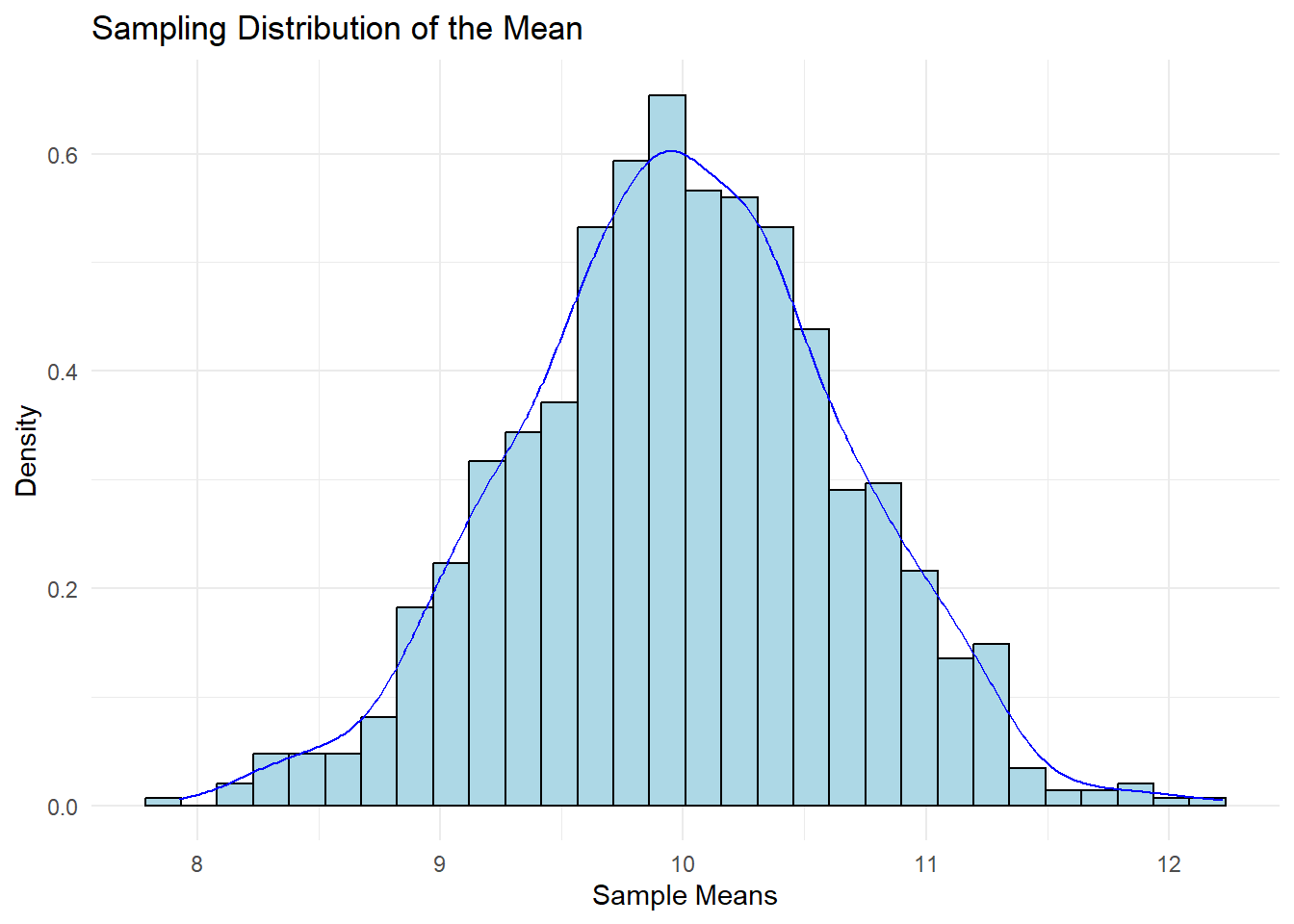

9.8 Confidence Intervals

Confidence intervals are a range of values within which the true population parameter is likely to fall, with a specified level of confidence (e.g., 95%). Confidence intervals provide an estimate of the precision and uncertainty of the sample statistic.

# Define the sample data
sample_data <- c(12, 15, 18, 20, 22, 24, 25, 28, 30, 32)

# Calculate the sample mean and standard deviation
sample_mean <- mean(sample_data)
sample_sd <- sd(sample_data)

# Calculate the standard error
standard_error <- sample_sd / sqrt(length(sample_data))

# Calculate the 95% confidence interval
alpha <- 0.05
critical_value <- qnorm(1 - alpha / 2)
margin_of_error <- critical_value * standard_error
confidence_interval <- c(sample_mean - margin_of_error, sample_mean + margin_of_error)