10 Hypothesis Testing
Hypothesis testing is a method used to make decisions about population parameters based on sample data.
10.1 Hypothesis
A hypothesis is an educated guess or statement about the relationship between variables or the characteristics of a population. In hypothesis testing, there are two main hypotheses:
10.2 Decision Type Error
When performing hypothesis testing, there are two types of decision errors:
Type I Error (α): This error occurs when the null hypothesis is rejected when it is actually true. In other words, it’s a false positive. The probability of committing a Type I error is denoted by the significance level (α), which is typically set at 0.05 or 0.01. Type II Error (β): This error occurs when the null hypothesis is not rejected when it is actually false. In other words, it’s a false negative. The probability of committing a Type II error is denoted by β. The power of a test (1 - β) measures the ability of the test to detect an effect when it truly exists. Here is a graphical representation of the types of decision errors:
Hypothesis Testing Errors
|                  | Null Hypothesis (H0) is True | Null Hypothesis (H0) is False |
|------------------|------------------------------|-------------------------------|
| Reject H0        | Type I Error (α)             | Correct Decision (1 - β)      |
| Fail to Reject H0| Correct Decision (1 - α)     | Type II Error (β)             |
This table represents the different outcomes when making decisions based on hypothesis testing. The columns represent the reality (i.e., whether the null hypothesis is true or false), and the rows represent the decision made based on the hypothesis test (i.e., whether to reject or not reject the null hypothesis). The cells show the types of decision errors (Type I and Type II errors) and the correct decisions.
10.3 Level of Signficance
The level of significance is a critical component in hypothesis testing because it sets a threshold for determining whether an observed effect is statistically significant or not.
The level of significance is denoted by the Greek letter α (alpha) and represents the probability of making a Type I error. A Type I error occurs when we reject the null hypothesis (H0) when it is actually true. By choosing a level of significance, researchers define the risk they are willing to take when rejecting a true null hypothesis. Common levels of significance are 0.05 (5%) and 0.01 (1%).
To better understand the role of the level of significance in hypothesis testing, let’s consider the following steps:
Formulate the null hypothesis (H0) and the alternative hypothesis (H1): The null hypothesis typically states that there is no effect or relationship between variables, while the alternative hypothesis states that there is an effect or relationship.
Choose a level of significance (α): Determine the threshold for the probability of making a Type I error. For example, if α is set to 0.05, there is a 5% chance of rejecting a true null hypothesis.
Perform the statistical test and calculate the test statistic: The test statistic is calculated using the sample data, and it helps determine how far the observed sample mean is from the hypothesized population mean. In the case of a single mean, a one-sample t-test is commonly used, and the test statistic is the t-value.
Determine the critical value or p-value: Compare the calculated test statistic with the critical value or the p-value (probability value) to make a decision about the null hypothesis. The critical value is a threshold value that depends on the chosen level of significance and the distribution of the test statistic. The p-value represents the probability of obtaining a test statistic as extreme or more extreme than the observed test statistic under the assumption that the null hypothesis is true.
Make a decision: If the test statistic is more extreme than the critical value, or if the p-value is less than the level of significance (α), reject the null hypothesis. Otherwise, fail to reject the null hypothesis.
10.4 T-statistic
The t-statistic is a standardized measure used in hypothesis testing to compare the observed sample mean with the hypothesized population mean. It takes into account the sample mean, the hypothesized population mean, and the standard error of the mean. Mathematically, the t-statistic can be calculated using the following formula:
t = (X̄ - μ) / (s / √n)
where:
t is the t-statistic X̄ is the sample mean μ is the hypothesized population mean s is the sample standard deviation n is the sample size
10.4.1 T-distribution
The t-distribution, also known as the Student’s t-distribution, is a probability distribution that is used when the population standard deviation is unknown and the sample size is small. It is similar to the normal distribution but has thicker tails, which accounts for the increased variability due to using the sample standard deviation as an estimate of the population standard deviation. The shape of the t-distribution depends on the degrees of freedom (df), which is related to the sample size (df = n - 1). As the sample size increases, the t-distribution approaches the normal distribution.
To calculate the t-statistic in R, you can use the following code:
# Sample data
data <- c(12, 14, 16, 18, 20)

# Hypothesized population mean
hypothesized_mean <- 15

# Calculate the sample mean, standard deviation, and size
sample_mean <- mean(data)
sample_sd <- sd(data)
sample_size <- length(data)

# Calculate the t-statistic
t_statistic <- (sample_mean - hypothesized_mean) / (sample_sd / sqrt(sample_size))

# Print the t-statistic
print(t_statistic)
#> [1] 0.7071068
To perform a one-sample t-test in R, which calculates the t-statistic and p-value automatically, you can use the t.test() function:
# Perform a one-sample t-test
t_test_result <- t.test(data, mu = hypothesized_mean)

# Print the t-test result
print(t_test_result)
#>
#>  One Sample t-test
#>
#> data:  data
#> t = 0.70711, df = 4, p-value = 0.5185
#> alternative hypothesis: true mean is not equal to 15
#> 95 percent confidence interval:
#>  12.07351 19.92649
#> sample estimates:
#> mean of x
#>        16
10.4.2 Intepreting Normality Evidence
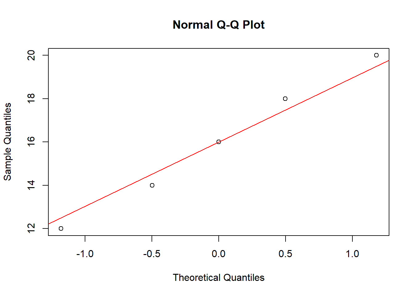
When using a t-test, the assumption of normality is important. The data should follow a normal distribution to ensure the validity of the test results. To assess the normality of the data, we can use visual methods (histograms, Q-Q plots) and statistical tests (e.g., Shapiro-Wilk test).
This is important because the t-test assumes that the data follow a normal distribution, and verifying this assumption helps ensure the validity of the test results.
To generate normality evidence after performing a t-test, you can use the following methods:
Visual methods: Histograms and Q-Q plots can provide a visual assessment of the normality of the data.
Statistical tests: Shapiro-Wilk test and Kolmogorov-Smirnov test are commonly used to test for normality. These tests generate p-values, which can be compared with a chosen significance level (e.g., 0.05) to determine if the data deviate significantly from normality.
In R, you can create a histogram and Q-Q plot using the following code:
- Create a histogram and Q-Q plot:
# Load required libraries
library(ggplot2)
#> Warning: package 'ggplot2' was built under R version 4.2.3

# Sample data
data <- c(12, 14, 16, 18, 20)

# Create a histogram
ggplot(data.frame(data), aes(data)) +
  geom_histogram(binwidth = 1, color = "black", fill = "white") +
  theme_minimal()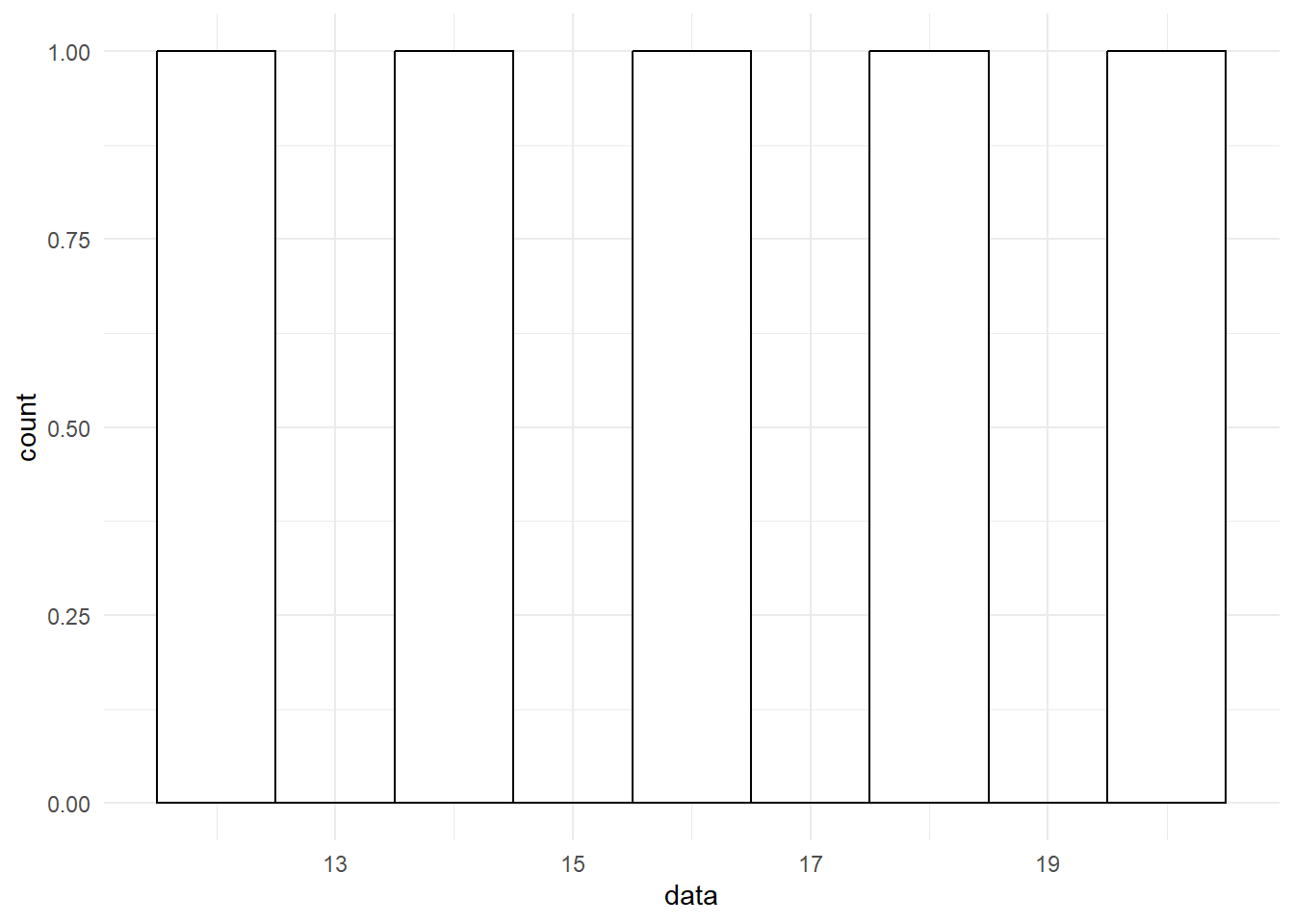
- Perform the Shapiro-Wilk test:
# Perform the Shapiro-Wilk test
shapiro_test_result <- shapiro.test(data)

# Print the test result
print(shapiro_test_result)
#>
#>  Shapiro-Wilk normality test
#>
#> data:  data
#> W = 0.98676, p-value = 0.9672
To interpret the normality evidence, follow these guidelines:
Visual methods: Inspect the histogram and Q-Q plot. If the histogram is roughly bell-shaped and the points on the Q-Q plot fall approximately on the reference line, the data can be considered approximately normally distributed.
Statistical tests: Check the p-values of the normality tests. If the p-value is greater than the chosen significance level (e.g., 0.05), the null hypothesis (i.e., the data follow a normal distribution) cannot be rejected. This suggests that the data do not deviate significantly from normality.
Keep in mind that no single method is foolproof, and it’s often a good idea to use a combination of visual and statistical methods to assess normality. If the data appear to be non-normal, you might consider using non-parametric alternatives to the t-test or transforming the data to achieve normality.
10.5 Statistical Power
Statistical power is the probability of correctly rejecting the null hypothesis when it is false, which means not committing a Type II error. Power is influenced by factors such as sample size, effect size, and the chosen significance level (α). Power analysis helps researchers determine the appropriate sample size needed to achieve a desired level of power, typically 0.8 or higher.
To perform power analysis in R, you can use the pwr package, which provides a set of functions for power calculations in various statistical tests, including the t-test.
Here’s a step-by-step procedure for generating and testing power using R:
- Install and load the pwr package:
- Define the parameters for power analysis. You will need to specify the effect size (Cohen’s d), sample size, and significance level (α):
# Define parameters for power analysis
effect_size <- 0.8  # Cohen's d
sample_size <- 20
significance_level <- 0.05- Use the pwr.t.test() function to calculate the power for a one-sample t-test:
# Calculate the power for a one-sample t-test
power_result <- pwr.t.test(n = 500,
                           d = effect_size,
                           sig.level = significance_level,
                           type = "one.sample",
                           alternative = "two.sided")

# Print the power result
print(power_result)
#>
#>      One-sample t test power calculation
#>
#>               n = 500
#>               d = 0.8
#>       sig.level = 0.05
#>           power = 1
#>     alternative = two.sided
The output will show the calculated power, sample size, effect size, and significance level. If the power is below the desired level (e.g., 0.8), you can adjust the sample size or effect size and recalculate the power to determine the necessary changes for achieving the desired power level.
It’s essential to consider the practical implications of the effect size and sample size when planning a study. A large effect size may be easier to detect but might not occur frequently in real-world situations. Conversely, a small effect size might be more difficult to detect and may require a larger sample size to achieve adequate power.