Chapter 8 Matrix Completion Methods

Source RMD file: link

In this chapter, we continue looking into a setting where $N$ units are observed over $T$ periods as in Chapter 7. This time, we setup the problem using matrices and explain how existing methods - some of which we already covered in Chapter 7 - fit in this framework. We then introduce a matrix completion method proposed by Athey, Bayati, Doudchenko, Imbens, and Khosravi (2021).

# To install MCPanel package, uncomment the next lines as appropriate.
# install.packages("devtools")  # if you don't have this installed yet.
# library(devtools) 
# devtools::install_github("susanathey/MCPanel")
library(MCPanel)
library(ggplot2)
#install.packages("latex2exp")
library(latex2exp)

8.1 Set Up

Suppose we observe

$$Y =\left( \begin{array}{ccccccc} Y_{11} & Y_{12} & Y_{13} & \dots & Y_{1T} \\ Y_{21} & Y_{22} & Y_{23} & \dots & Y_{2T} \\ Y_{31} & Y_{32} & Y_{33} & \dots & Y_{3T} \\ \vdots & \vdots & \vdots &\ddots &\vdots \\ Y_{N1} & Y_{N2} & Y_{N3} & \dots & Y_{NT} \\ \end{array} \right)\hskip1cm {\rm (realized\ outcome)}.$$

$$W=\left( \begin{array}{ccccccc} 1 & 1 & 0 & \dots & 1 \\ 0 & 0 & 1 & \dots & 0 \\ 1 & 0 & 1 & \dots & 0 \\ \vdots & \vdots & \vdots &\ddots &\vdots \\ 1 & 0 & 1 & \dots & 0 \\ \end{array} \right)\hskip1cm {\rm (binary\ treatment)}.$$

where rows of $Y$ and $W$ correspond to physical units, while the columns correspond to time periods.

Throughout this chapter, the $\checkmark$ marks indicate the observed values and the $\color{red} ?$ marks indicate the missing values.

So in terms of potential outcome matrices $Y(0)$ and $Y(1)$, $Y_{it}(0)$ is observed iff $W_{it}=0$ while $Y_{it}(1)$ is observed iff $W_{it}=1$. So, the matrices look like the following: $$Y(0)=\left( \begin{array}{ccccccc} {\color{red} ?} & {\color{red} ?} & \checkmark & \dots & {\color{red} ?} \\ \checkmark & \checkmark & {\color{red} ?} & \dots & \checkmark \\ {\color{red} ?} & \checkmark & {\color{red} ?} & \dots & \checkmark \\ \vdots & \vdots & \vdots &\ddots &\vdots \\ {\color{red} ?} & \checkmark & {\color{red} ?} & \dots & \checkmark \\ \end{array} \right)\hskip1cm Y(1)=\left( \begin{array}{ccccccc} \checkmark & \checkmark & {\color{red} ?} & \dots & \checkmark \\ {\color{red} ?} & {\color{red} ?} & \checkmark & \dots & {\color{red} ?} \\ \checkmark & {\color{red} ?} & \checkmark & \dots & {\color{red} ?} \\ \vdots & \vdots & \vdots &\ddots &\vdots \\ \checkmark & {\color{red} ?} &\checkmark & \dots & {\color{red} ?} \\ \end{array} \right).$$

In order to estimate the treatment effect for the treated, $$\tau=\frac{\sum_{i,t} W_{it} \Biggl(Y_{it}(1)-Y_{it}(0)\Biggr)}{\sum_{it} W_{it}},$$

We would need to impute the missing potential outcomes in $Y(0)$. We might to need impute the missing potential outcomes in $Y(1)$ if we are interested in some other estimand.

In this chapter, we focus on problem of imputing missing values in $N \times T$ matrix $Y(0)$. Let’s denote it by $Y_{N\times T}$ where

$${Y_{N\times T}}=\left( \begin{array}{ccccccc} {\color{red} ?} & {\color{red} ?} & \checkmark & \dots & {\color{red} ?} \\ \checkmark & \checkmark & {\color{red} ?} & \dots & \checkmark \\ {\color{red} ?} & \checkmark & {\color{red} ?} & \dots & \checkmark \\ \vdots & \vdots & \vdots &\ddots &\vdots \\ {\color{red} ?} & \checkmark & {\color{red} ?} & \dots & \checkmark \\ \end{array} \right).$$

This problem is now a matrix completion problem.

Throughout this chapter, we use the following notation. Let

• $\cal{M}$ denote the set of pairs of indices $(i,t)\in [N]\times[T]$, corresponding to the missing entries (in the above case, the entries with $W_{it} = 1$)
• $\cal{O}$ denote the set of pairs of indices corresponding to the observed entries (in the above case, the entries with $W_{it} = 0$).

8.2 Patterns of missing data

In social science applications, the missingness arises from treatment assignments and the choices that lead to these assignments. As a result, there are often specific structures on the missing data.

8.2.1 Block structure

A leading example is a block structure, with a subset of the units adopting an irreversible treatment at a particular point in time $T_0+1$.

$${Y_{N\times T}}=\left( \begin{array}{ccccccc} \checkmark & \checkmark & \checkmark & \checkmark & \dots & \checkmark \\ \checkmark & \checkmark & \checkmark & \checkmark & \dots & \checkmark \\ \checkmark & \checkmark & \checkmark & \checkmark & \dots & \checkmark \\ \checkmark & \checkmark & \checkmark & {\color{red} ?} & \dots & {\color{red} ?} \\ \checkmark & \checkmark & \checkmark & {\color{red} ?} & \dots & {\color{red} ?} \\ \vdots & \vdots & \vdots & \vdots & \ddots &\vdots \\ \checkmark & \checkmark & \checkmark & {\color{red} ?} & \dots & {\color{red} ?} \\ \\ \end{array} \right)$$

There are two special cases of the block structure. Much of the literature on estimating average treatment effects under unconfoundedness focuses on the case where $T_0=T-1$, so that the only treated units are in the last period. We will refer to this as the single-treated-period block structure.

$${Y_{N\times T}}=\left( \begin{array}{ccccccc} \checkmark & \checkmark & \checkmark & \dots & \checkmark & \checkmark \\ \checkmark & \checkmark & \checkmark & \dots & \checkmark & \checkmark \\ \checkmark & \checkmark & \checkmark & \dots & \checkmark & {\color{red} ?} \\ \vdots & \vdots & \vdots & \ddots &\vdots &\vdots \\ \checkmark & \checkmark & \checkmark & \dots & \checkmark & {\color{red} ?} \\ &&&& & \uparrow \\ &&&& & {\rm treated\ period} \\ \end{array} \right).$$

In contrast, the synthetic control literature primarily focuses on the case with a single treated unit which are treated for a number of periods from period $T_0+1$ onwards. We will refer to this as the single-treated-unit block structure.

$${Y_{N\times T}}=\left( \begin{array}{ccccccc} \checkmark & \checkmark & \checkmark & \dots & \checkmark \\ \checkmark & \checkmark & \checkmark & \dots & \checkmark \\ \checkmark & \checkmark & \checkmark & \dots & \checkmark \\ \vdots & \vdots & \vdots & \ddots &\vdots\\ \checkmark & \checkmark & \checkmark & \dots & \checkmark \\ \checkmark & \checkmark & {\color{red} ?} & \dots & {\color{red} ?} & \leftarrow & {\rm treated\ unit} \\ \end{array} \right).$$

A special case that fits in both these settings is that with a single missing unit/time pair. This specific setting is useful to contrast methods developed for the single-treated-period case (unconfoundedness) and the single-treated-unit case (synthetic control) because both sets of methods are potentially applicable.

$${Y_{N\times T}}=\left( \begin{array}{ccccccc} \checkmark & \checkmark & \checkmark & \dots & \checkmark & \checkmark \\ \checkmark & \checkmark & \checkmark & \dots & \checkmark & \checkmark \\ \checkmark & \checkmark & \checkmark & \dots & \checkmark & \checkmark \\ \vdots & \vdots & \vdots & \ddots &\vdots &\vdots \\ \checkmark & \checkmark & \checkmark & \dots & \checkmark & \checkmark \\ \checkmark & \checkmark & \checkmark & \dots & \checkmark & {\color{red} ?} \\ \end{array} \right).$$

8.2.2 Staggered Adoption

Another setting to be considered is the Staggered Adoption design. In this design, each unit is characterized by an adoption date $T_i \in \{1, ...,T,\infty\}$ which is the first date they are exposed to the treatment. Once they are exposed to the treatment, the treatment is irreversible. This naturally arises where the treatment is some new technology that units can choose to adopt.

$$Y_{N\times T}=\left( \begin{array}{ccccccr} \checkmark & \checkmark & \checkmark & \checkmark & \dots & \checkmark & {\rm (never\ adopter)}\\ \checkmark & \checkmark & \checkmark & \checkmark & \dots & {\color{red} ?} & {\rm (late\ adopter)}\\ \checkmark & \checkmark & \checkmark & \checkmark & \dots & {\color{red} ?} \\ \checkmark & \checkmark &{\color{red} ?} & {\color{red} ?} & \dots & {\color{red} ?} \\ \checkmark & \checkmark & {\color{red} ?} & {\color{red} ?} & \dots & {\color{red} ?} &\ \ \ {\rm (medium\ adopter)} \\ \vdots & \vdots & \vdots & \vdots &\ddots &\vdots \\ \checkmark & {\color{red} ?} & {\color{red} ?} & {\color{red} ?} & \dots & {\color{red} ?} & {\rm (early\ adopter)} \\ \end{array} \right)$$

8.3 Thin and Fat Matrices

The relative size of $N$ and $T$ gives us the possible shape of the data matrices. Relative to the number of time periods, we may have many units, few units or a comparable number of units.

So Y can be a thin matrix where the number of columns is much smaller than the number of rows: $${Y_{N\times T}}=\left( \begin{array}{ccccccc} {\color{red} ?} & {\color{red} ?} & \checkmark \\ \checkmark & \checkmark & {\color{red} ?} \\ {\color{red} ?} & \checkmark & {\color{red} ?} \\ \vdots & \vdots & \vdots \\ {\color{red} ?} & \checkmark & {\color{red} ?} \\ \end{array} \right) (N \gg T).$$

Or Y can be a fat matrix where the number of columns is much bigger than the number of rows:

$${Y_{N\times T}}=\left( \begin{array}{ccccccc} {\color{red} ?} & {\color{red} ?} & \checkmark & \checkmark& \dots & {\color{red} ?} \\ \checkmark & \checkmark & {\color{red} ?} & \checkmark & \dots & \checkmark \\ {\color{red} ?} & \checkmark & {\color{red} ?} & {\color{red} ?} & \dots & \checkmark \\ \end{array} \right) (N \ll T).$$

Or Y can be an approximately square matrix where the number of columns is approximately equal to the number of rows:

$${Y_{N\times T}}=\left( \begin{array}{ccccccc} {\color{red} ?} & {\color{red} ?} & \checkmark & \dots & {\color{red} ?} \\ \checkmark & \checkmark & {\color{red} ?} & \dots & \checkmark \\ {\color{red} ?} & \checkmark & {\color{red} ?} & \dots & \checkmark \\ \vdots & \vdots & \vdots & \ddots & \vdots \\ {\color{red} ?} & \checkmark & {\color{red} ?} & \dots & \checkmark \\ \end{array} \right) (N \approx T).$$

8.4 Horizontal and Vertical Regressions

8.4.1 Horizontal Regression and Unconfoundedness literature

The unconfoundedness literature focuses on the single-treated-period structure with a thin matrix ($N \gg T$), a substantial number of treated and control units, and imputes the missing potential outcomes using control units with similar lagged outcomes.

So $Y_{iT}$ is missing for some $i$ ($N_t$ “treated units”) and no missing entries for other units ($N_c = N - N_t$ “control units”):

$$Y_{N\times T}=\left( \begin{array}{ccccccc} \checkmark & \checkmark & \checkmark \\ \checkmark & \checkmark & \checkmark \\ \checkmark & \checkmark & {\color{red} ?} \\ \checkmark & \checkmark & {\color{red} ?} \\ \checkmark & \checkmark & \checkmark \\ \vdots & \vdots &\vdots \\ \checkmark & \checkmark & {\color{red} ?} \\ \end{array} \right)\hskip1cm W_{N\times T}=\left( \begin{array}{ccccccc} 1 & 1 & 1 \\ 1 & 1 & 1 \\ 1 & 1 & 0 \\ 1 & 1 & 0 \\ 1 & 1 & 1 \\ \vdots & \vdots &\vdots \\ 1 & 1 & 0 \\ \end{array} \right)$$

Recall that $\cal{M}$ denotes the set of pairs of indices $(i,t)$, corresponding to the missing entries and $\cal{O}$ denotes the set of pair of indices corresponding to the observed entries. In this setting, the identification depends on the assumption that:

$$Y_{i,T}(0) \perp \!\!\! \perp W_{i,T} | Y_{i,1}, ...., Y_{i,T-1},$$

for the units with $(i,t)\in \cal{M}$, i.e., the units that have missing entries.

A simple version of the unconfoundedness approach is to regress the last period outcome on the lagged outcomes and use the estimated regression to predict the missing potential outcomes. That is, for the units with $(i,t)\in \cal{M}$, the predicted outcome is:

$$\hat Y_{iT}=\hat \beta_0+\sum_{s=1}^{T-1} \hat \beta_s Y_{Nt},$$

where

$$\hat\beta= \arg\min_{\beta} \sum_{i:(i,T)\in \cal{O}}(Y_{iT}-\beta_0-\sum_{s=1}^{T-1}\beta_s Y_{is})^2.$$

This is referred to as horizontal regression, where the rows of the $Y$ matrix form the units of observation. A more flexible, nonparametric, version of this estimator would correspond to matching, where for each treated unit $i$ we find a corresponding control unit $j$ with $Y_{jt} \approx Y_{it}$ for all pre-treatment periods $t = 1,..., T − 1$. If $N$ is large relative to $T_0$, use regularized regression such as lasso, ridge, and elastic net.

8.4.2 Vertical Regression and the Synthetic Control literature

The synthetic control methods, which we introduced in Chapter 7, focus primarily on the single-treated-unit block structure with a relatively fat ($T\gg N$) or approximately square ($T\approx N$) and a substantial number of pre-treatment periods. $Y_{Nt}$ is missing for $t \geq T_0$ and there are no missing entries for other units:

$$Y_{N\times T}=\left( \begin{array}{ccccccc} \checkmark & \checkmark & \checkmark & \dots & \checkmark \\ \checkmark & \checkmark & \checkmark & \dots & \checkmark \\ \checkmark & \checkmark & {\color{red} ?} & \dots & {\color{red} ?} \\ \end{array} \right)\hskip0.5cm W_{N\times T}=\left( \begin{array}{ccccccc} 1 & 1 & 1 & \dots & 1 \\ 1 & 1 & 1 & \dots & 1 \\ 1 & 1 & 0 & \dots & 0 \\ \end{array} \right)$$

In this setting, the identification depends on the assumption that:

$$Y_{N,t}(0) \perp \!\!\! \perp W_{N,T} | Y_{1,t}, ...., Y_{N-1,T}.$$

Doudchenko and Imbens (2016) and Ferman and Pinto (2021) show how the Abadie-Diamond-Hainmueller synthetic control method can be interpreted as regressing the outcomes for the treated unit prior to the treatment on the outcomes for the control units in the same periods. That is, for the treated unit in period $t$, for $t=T_0, ..., T$, the predicted outcome is:

$$\hat Y_{Nt}=\hat \omega_0+\sum_{i=1}^{N-1} \hat \omega_i Y_{it}$$

where

$$\hat\omega= \arg\min_{\omega} \sum_{t:(N,t)\in \cal{O}}(Y_{Nt}-\omega_0-\sum_{i=1}^{N-1}\omega_i Y_{is})^2.$$

This is referred to as vertical regression where the columns of the $Y$ matrix form the units of observation. A more flexible, nonparametric, version of this estimator would correspond to matching, where for each post-treatment period $t$ we find a corresponding pre-treatment period $s$ with $Y_{is} \approx Y_{it}$ for all control units $i = 1,..., N − 1$. If $T$ is large relative to $N_c$, one could use regularized regression such as lasso, ridge, and elastic net, following Doudchenko and Imbens (2016).

8.5 Fixed Effects and Factor models

8.5.1 Panel with Fixed Effects

The horizontal regression focuses on a pattern in the time path of the outcome $Y_{it}$, specifically the relation between $Y_{iT}$ and the lagged $Y_{it}$ for $t = 1,..., T-1$ for the units for whom these values are observed, and assumes that this pattern is the same for units with missing outcomes. The vertical regression focuses on a pattern between units at times when we observe all outcomes, and assumes this pattern continues to hold for periods when some outcomes are missing. However, by focusing on only one of these patterns, cross-section or time series, these approaches ignore alternative patterns that may help in imputing the missing values. One alternative is to consider approaches that allow for the exploitation of stable patterns over time and stable patterns across units. Such methods have a long history in panel data literature, including the two-way fixed effects, and factor and interactive mixed effect models.

In the absence of covariates, the common two-way fixed effect model is: $$Y_{it} = \delta_i + \gamma_t + \epsilon_{it}.$$

In this setting, the identification depends on the assumption that:

$$Y_{i,t}(0) \perp \!\!\! \perp W_{i,T} | \delta_i, \gamma_t.$$

So the predicted outcome based on the unit and time fixed effects is: $$\hat{y}_{NT} = \hat{\delta}_N + \hat{\gamma}_T.$$

In a matrix form, the model can be rewritten as: $$Y_{N\times T}= L_{N \times T} + \epsilon_{N \times T} = \left( \begin{array}{ccccccc} \delta_1 & 1 \\ \vdots & \vdots \\ \delta_N & 1 \\ \end{array}\right) \left( \begin{array}{ccccccc} 1 & \dots & 1 \\ \gamma_1 & \dots & \gamma_T \\ \end{array} \right) + \epsilon_{N \times T}$$

The matrix formulation of the identification assumption is:

$$Y_{N\times T}(0) \perp \!\!\! \perp W_{N \times T} | L_{N \times T}.$$

8.5.2 Interactive Fixed Effects

For interactive fixed effects, instead of exploiting additive structure in unit and time effects, we exploit the low rank or interactive structure of unit and time fixed effects for panel data regression.

The common interactive fixed effect model is:

$$Y_{it} = \sum_{r=1}^{R} \delta_{ir}\gamma_{rt} + \epsilon_{it},$$

where $\delta_{ir}$ are called factors and $\gamma_{rt}$ are called factor loadings. Note that both factors and factor loadings are parameters that need to be estimated. Typically it is assumed that the number of factors $R$ is fixed, although it is not necessarily known to the researcher. See e.g., Bai and Ng (2002) and Moon and Weidner (2015) on estimating the number of factors $R$.

Again, the identification depends on the assumption that:

$$Y_{i,t}(0) \perp \!\!\! \perp W_{i,T} | \delta_i, \gamma_t.$$

The predicted outcome based on the interactive fixed effects would be: $\hat{y}_{NT} = \sum_{r=1}^{R} \hat{\delta}_{ir}\hat{\gamma}_{rt}$

In a matrix form, the $Y_{N \times T}$ can be rewritten as: $$Y_{N\times T}=L_{N \times T} + \epsilon_{N \times T} = \left( \begin{array}{ccccccc} \delta_{11} & \dots & \delta_{R1} \\ \vdots & \dots & \vdots \\ \vdots & \dots & \vdots \\ \vdots & \dots & \vdots \\ \delta_{1N} & \dots & \delta_{RN} \\ \end{array}\right) \left( \begin{array}{ccccccc} \gamma_{11} & \dots \dots \dots & \gamma_{1T} \\ \vdots & \dots \dots \dots & \vdots \\ \gamma_{R1} & \dots \dots \dots & \gamma_{RT} \\ \end{array} \right) + \epsilon_{N \times T}$$

The matrix formulation of the identification assumption is:

$$Y_{N\times T}(0) \perp \!\!\! \perp W_{N \times T} | L_{N \times T}.$$

Using the interactive fixed effects model, we would estimate $\delta$ and $\gamma$ by least squares regression and use those to impute missing values.

8.6 Machine Learning on Matrix Completion

The machine learning literature on matrix completion focuses on a setting where there are many missing entries such that $|\cal{O}|/|\cal{M}| \approx 0$. It focuses on the case with randomly missing entries, i.e., $W \perp \!\!\! \perp Y$. Examples include the Netflix problem with units corresponding to individuals, and time periods corresponding to movie titles or image recovery from limited information, with $i$ and $t$ corresponding to different dimensions. So the matrix $Y$ looks like the following where it has a general missing data pattern and the fraction of observed data to missing data is close to zero:

$$Y_{N\times T}=\left( \begin{array}{cccccccccc} {\color{red} ?} & {\color{red} ?} & {\color{red} ?} & {\color{red} ?} & {\color{red} ?}& \checkmark & \dots & {\color{red} ?}\\ \checkmark & {\color{red} ?} & {\color{red} ?} & {\color{red} ?} & \checkmark & {\color{red} ?} & \dots & \checkmark \\ {\color{red} ?} & \checkmark & {\color{red} ?} & {\color{red} ?} & {\color{red} ?} & {\color{red} ?} & \dots & {\color{red} ?} \\ {\color{red} ?} & {\color{red} ?} & {\color{red} ?} & {\color{red} ?} & {\color{red} ?}& \checkmark & \dots & {\color{red} ?}\\ \checkmark & {\color{red} ?} & {\color{red} ?} & {\color{red} ?} & {\color{red} ?} & {\color{red} ?} & \dots & \checkmark \\ {\color{red} ?} & \checkmark & {\color{red} ?} & {\color{red} ?} & {\color{red} ?} & {\color{red} ?} & \dots & {\color{red} ?} \\ \vdots & \vdots & \vdots &\vdots & \vdots & \vdots &\ddots &\vdots \\ {\color{red} ?} & {\color{red} ?} & {\color{red} ?} & {\color{red} ?}& \checkmark & {\color{red} ?} & \dots & {\color{red} ?}\\ \end{array} \right)$$

The literature also focuses on computational feasibility as both $N$ and $T$ are large.

8.6.1 The Matrix Completion with Nuclear Norm Minimization Estimator

Following Athey, Bayati, Doudchenko, Imbens, and Khosravi (2021), we set up the model as follows.

In the absence of covariates, the $Y_{N \times T}$ matrix can be rewritten as

$$Y_{N\times T}=L_{N \times T} + \epsilon_{N \times T}.$$

The key assumptions are:

• $W_{N\times T} \perp \!\!\! \perp\varepsilon_{N\times T}$ (but $W$ may depend on $L$).
• there exists staggered entry relating to the weights such that $W_{it+1} \geq W_{it}$ and
• $L$ has a low rank relative to $N$ and $T$.

In a more general case with unit-specific $P$-component covariate $X_i$, time-specific $Q$-component covariate $Z_t$, and unit-time-specific covariate $V_{it}$, $Y_{it}$ is equal to: $$Y_{it} = L_{it}+\sum_{p=1}^P \sum_{q=1}^Q X_{ip} H_{pq} Z_{qt}+\gamma_i+\delta_t+V_{it}\beta +\varepsilon_{it}$$

We do not necessarily need the fixed effects $\gamma_i$ and $\delta_t$ as these can be subsumed into $L$. However, it is convenient to include the fixed effects given that we regularize $L$.

With too many parameters, especially for $N\times T$ matrix $L$, we need regularization such that we shrink $L$ and $H$ toward zero. To regularize H, we use Lasso-type element-wise $\ell_1$ norm, defined as $\|H\|_{1,e}=\sum_{p=1}^P \sum_{q=1}^Q |H_{pq}|$.

But how do we regularize $L$?

$L_{N \times T}$ is equal to: $$L_{N\times T}=S_{N\times N} \Sigma_{N\times T} R_{T\times T}$$ where $S$, $R$ unitary, $\Sigma$ is rectangular diagonal with entries $\sigma_i(L)$ that are the singular values. Rank of $L$ is number of non-zero $\sigma_i(L)$.

There are three ways to regularize L: $$\|L\|_F^2=\sum_{i,t}|L_{it}|^2=\sum_{j=1}^{\min(N,T)}\sigma^2_i(L)\hskip1cm {\rm (Frobenius,\ like\ ridge)}$$ $$\|L\|_{*}=\sum_{j=1}^{\min(N,T)}\sigma_i(L)\hskip1cm {\rm \bf (nuclear\ norm,\ like\ LASSO)}$$ $$\|L\|_R=\sum_{j=1}^{\min(N,T)}{\bf 1}_{\sigma_i(L)>0}\hskip1cm {\rm (Rank,\ like\ subset\ selection)}$$

Frobenius norm imputes missing values as 0. Rank norm is computationally not feasible for general missing data patterns. The preferred Nuclear norm leads to low-rank matrix but is computationally feasible.

So the Matrix-Completion with Nuclear Norm Minimization (MC-NNM) estimator uses the nuclear norm: $$\min_{L}\frac{1}{|\cal{O}|} \sum_{(i,t) \in \cal{o}} \left(Y_{it} - L_{it} \right)^2+\lambda_L \|L\|_*$$

For the general case, we estimate $H$, $L$, $\delta$, $\gamma$, and $\beta$ as $$\min_{H,L,\delta,\gamma}\frac{1}{|\cal{O}|} \sum_{(i,t) \in \cal{O}} \left(Y_{it} - L_{it}-\sum_{p=1}^P \sum_{q=1}^Q X_{ip} H_{pq} Z_{qt}-\gamma_i-\delta_t-V_{it}\beta \right)^2 +\lambda_L \|L\|_* + \lambda_H \|H\|_{1,e}$$

And we choose $\lambda_L$ and $\lambda_H$ through cross-validation.

A major advantage of using the nuclear norm is that the resulting estimator can be computed using fast convex optimization programs, such as the SOFT-IMPUTE algorithm by Mazumder, Hastie, & Tibshirani (2010). To describe it, we first introduce some notations. Given any $N\times T$ matrix $A$, define the two $N\times T$ matrices $P_\cal{O}(A)$ and $P_\cal{O}^\perp(A)$ with typical elements: $$P_\cal{O}(A)_{it}= \left\{ \begin{array}{ll} A_{it}\hskip1cm & {\rm if}\ (i,t)\in\cal{O}\,,\\ 0&{\rm if}\ (i,t)\notin\cal{O}\,, \end{array}\right.$$ and $$P_\cal{O}^\perp(A)_{it}= \left\{ \begin{array}{ll} 0\hskip1cm & {\rm if}\ (i,t)\in\cal{O}\,,\\ A_{it}&{\rm if}\ (i,t)\notin\cal{O}\,. \end{array}\right.$$ Let $A=S\Sigma R^\top$ be the Singular Value Decomposition for $A$, with $\sigma_1(A),\ldots,\sigma_{\min(N,T)}(A)$, denoting the singular values. Then define the matrix shrinkage operator $$\ shrink_\lambda(A)=S \tilde\Sigma R^\top\,,$$ where $\tilde\Sigma$ is equal to $\Sigma$ with the $i$-th singular value $\sigma_i(A)$ replaced by $\max(\sigma_i(A)-\lambda,0)$.

Given these definitions, the algorithm proceeds as follows.

1. Start with the initial choice $L_1(\lambda)=P_\cal{O}(Y)$, with zeros for the missing values.

2. Then for $k=1,2,\ldots,$ define, $$L_{k+1}(\lambda)=shrink_\lambda\Biggl\{P_\cal{O}(Y)+P_\cal{O}^\perp\Big(L_k(\lambda)\Big)\Biggr\}\,$$ until the sequence $\left\{L_k(\lambda)\right\}_{k\ge 1}$ converges.

3. The limiting matrix $L^*$ is our estimator for the regularization parameter $\lambda$, denoted by $\hat{L}(\lambda,\cal{O})$.

Here are the results following regularization for the case without covariates and just $L$, $\cal{O}$ is sufficiently random, and $\varepsilon_{it}=Y_{it}-L_{it}$ are iid with variance $\sigma^2$.

Let $\|Y\|_F=\sqrt{\sum_{i,t}Y_{i,t}^2}$ be Frobenius norm and $\|Y\|_\infty=\max_{i,t}|Y_{i,t}|$. Let $Y^*$ be the matrix including all the missing values (e.g., $Y(1)$). The estimated matrix $\hat{L}$ is close to $L^*$ in the following sense: $$\frac{\left\| \hat{L}-L\right\|_F}{\left\|L\right\|_F} \leq C\,\max\left(\sigma, \frac{\left\| L\right\|_\infty}{\left\|L\right\|_F}\right) \frac{{\rm rank}(L)(N+T)\ln(N+T)}{|\cal{O}| }$$

In many cases the number of observed entries $|\cal{O}|$ is of order $N\times T$ so if rank$(L)\ll (N+T)$ the error goes to $0$ as $N+T$ grows. Finally, note that the algorithm can be applied to a setting with covariates as well. Check Section 8 of Athey, Bayati, Doudchenko, Imbens, and Khosravi (2021) for more details.

8.6.2 Illustration

We compare the accuracy of imputation for the matrix completion method with previously used methods. In particular, in a real data matrix $Y$ where no unit is treated (no entries in the matrix are missing), we choose a subset of units as hypothetical treated units and aim to predict their values (for time periods following a randomly selected initial time). Then, we report the average root-mean-squared-error (RMSE) of each algorithm on values for the pseudo-treated (time, period) pairs. In these cases there is not necessarily a single right algorithm. Rather, we wish to assess which of the algorithms generally performs well, and which ones are robust to a variety of settings, including different adoption regimes and different configurations of the data.

We compare the following 5 estimators, using the California smoking data from the previous chapter:

• DID: Difference-in-differences based on regressing the observed outcomes on unit and time fixed effects and a dummy for the treatment.
• VT-EN: The vertical regression with elastic net regularization, relaxing the restrictions from the synthetic control estimator.
• HR-EN: The horizontal regression with elastic net regularization, similar to unconfoundedness type regressions.
• SC-ADH: The original synthetic control approach by Abadie et al. (2010), based on the vertical regression with Abadie-Diamond-Hainmueller restrictions. Although this estimator is not necessarily well-defined if $N\gg T$, the restrictions ensured that it was well-defined in all the settings we used.
• MC-NNM: Matrix-Completion Nuclear Norm Minimization estimator

We consider two settings for the treatment adoption:

• Case 1: Simultaneous adoption where randomly selected $N_t$ units adopt the treatment in period $T_0+1$, and the remaining units never adopt the treatment.
• Case 2: Staggered adoption where randomly $N_t$ units adopt the treatment in some period after $T$, with the actual adoption date varying randomly among these units.

First we will read in the data.

X <- read.csv('https://drive.google.com/uc?export=download&id=1b-jfaWF18m4G6DNYeTJrkx9zjG83Gt9n',header=F)
Y <- t(read.csv('https://drive.google.com/uc?export=download&id=12QfMzIABPWZJUnX-_May178zU-___EGU',header=F))
treat <- t(read.csv('https://drive.google.com/uc?export=download&id=1RCXwDJSSdQ2dvIH2XhEwK7ZOFQimYdQe',header=F))
years <- 1970:2000

And then set up other variables. Note that in the original data there are 39 units, but one of them (state of California) is treated. So we will remove California since the untreated values for that unit are not available. We then artificially designate some units and time periods to be treated and compare predicted values for those unit/time periods to the actual values.

In below code chunk, we consider staggered adoption (set is_simul$=1$ for simultaneous adoption).

## First row (treated unit)
CA_y <- Y[1,]

## Working with the rest of matrix
treat <- treat[-1,]
Y <- Y[-1,]

## Setting up the configuration
N <- nrow(treat)
T <- ncol(treat)
number_T0 <- 5
T0 <- ceiling(T*((1:number_T0)*2-1)/(2*number_T0))
N_t <- 35
num_runs <- 10

## Whether to simulate Simultaneous Adoption or Staggered Adoption
is_simul <- 0  ## 0 for Staggered Adoption and 1 for Simultaneous Adoption

# Matrices to save RMSE values 
MCPanel_RMSE_test <- matrix(0L,num_runs,length(T0))
EN_RMSE_test <- matrix(0L,num_runs,length(T0))
ENT_RMSE_test <- matrix(0L,num_runs,length(T0))
DID_RMSE_test <- matrix(0L,num_runs,length(T0))
ADH_RMSE_test <- matrix(0L,num_runs,length(T0))

Now, we calculate the RMSE values.

## Run different methods

for(i in c(1:num_runs)){
  print(paste0(paste0("Run number ", i)," started"))
  ## Fix the treated units in the whole run for a better comparison
  treat_indices <- sample(1:N, N_t)
  for (j in c(1:length(T0))){
    treat_mat <- matrix(1L, N, T);
    t0 <- T0[j]
    ## Simultaneuous (simul_adapt) or Staggered adoption (stag_adapt)
    if(is_simul == 1){
      treat_mat <- simul_adapt(Y, N_t, t0, treat_indices)
    }
    else{
      treat_mat <- stag_adapt(Y, N_t, t0, treat_indices)
    }
    Y_obs <- Y * treat_mat

    ## ------
    ## MC-NNM
    ## ------

    est_model_MCPanel <- mcnnm_cv(Y_obs, treat_mat, to_estimate_u = 1, to_estimate_v = 1)
    est_model_MCPanel$Mhat <- est_model_MCPanel$L + replicate(T,est_model_MCPanel$u) + t(replicate(N,est_model_MCPanel$v))
    est_model_MCPanel$msk_err <- (est_model_MCPanel$Mhat - Y)*(1-treat_mat)
    est_model_MCPanel$test_RMSE <- sqrt((1/sum(1-treat_mat)) * sum(est_model_MCPanel$msk_err^2))
    MCPanel_RMSE_test[i,j] <- est_model_MCPanel$test_RMSE

    ## -----
    ## EN : It does Not cross validate on alpha (only on lambda) and keep alpha = 1 (LASSO).
    ##      Change num_alpha to a larger number, if you are willing to wait a little longer.
    ## -----

    est_model_EN <- en_mp_rows(Y_obs, treat_mat, num_alpha = 1)
    est_model_EN_msk_err <- (est_model_EN - Y)*(1-treat_mat)
    est_model_EN_test_RMSE <- sqrt((1/sum(1-treat_mat)) * sum(est_model_EN_msk_err^2))
    EN_RMSE_test[i,j] <- est_model_EN_test_RMSE

    ## -----
    ## EN_T : It does Not cross validate on alpha (only on lambda) and keep alpha = 1 (LASSO).
    ##        Change num_alpha to a larger number, if you are willing to wait a little longer.
    ## -----
    est_model_ENT <- t(en_mp_rows(t(Y_obs), t(treat_mat), num_alpha = 1))
    est_model_ENT_msk_err <- (est_model_ENT - Y)*(1-treat_mat)
    est_model_ENT_test_RMSE <- sqrt((1/sum(1-treat_mat)) * sum(est_model_ENT_msk_err^2))
    ENT_RMSE_test[i,j] <- est_model_ENT_test_RMSE

    ## -----
    ## DID
    ## -----

    est_model_DID <- DID(Y_obs, treat_mat)
    est_model_DID_msk_err <- (est_model_DID - Y)*(1-treat_mat)
    est_model_DID_test_RMSE <- sqrt((1/sum(1-treat_mat)) * sum(est_model_DID_msk_err^2))
    DID_RMSE_test[i,j] <- est_model_DID_test_RMSE

    ## -----
    ## ADH
    ## -----
    est_model_ADH <- adh_mp_rows(Y_obs, treat_mat)
    est_model_ADH_msk_err <- (est_model_ADH - Y)*(1-treat_mat)
    est_model_ADH_test_RMSE <- sqrt((1/sum(1-treat_mat)) * sum(est_model_ADH_msk_err^2))
    ADH_RMSE_test[i,j] <- est_model_ADH_test_RMSE
  }
}

## [1] "Run number 1 started"
## [1] "Run number 2 started"
## [1] "Run number 3 started"
## [1] "Run number 4 started"
## [1] "Run number 5 started"
## [1] "Run number 6 started"
## [1] "Run number 7 started"
## [1] "Run number 8 started"
## [1] "Run number 9 started"
## [1] "Run number 10 started"

## Computing means and standard errors
MCPanel_avg_RMSE <- apply(MCPanel_RMSE_test,2,mean)
MCPanel_std_error <- apply(MCPanel_RMSE_test,2,sd)/sqrt(num_runs)

EN_avg_RMSE <- apply(EN_RMSE_test,2,mean)
EN_std_error <- apply(EN_RMSE_test,2,sd)/sqrt(num_runs)

ENT_avg_RMSE <- apply(ENT_RMSE_test,2,mean)
ENT_std_error <- apply(ENT_RMSE_test,2,sd)/sqrt(num_runs)

DID_avg_RMSE <- apply(DID_RMSE_test,2,mean)
DID_std_error <- apply(DID_RMSE_test,2,sd)/sqrt(num_runs)

ADH_avg_RMSE <- apply(ADH_RMSE_test,2,mean)
ADH_std_error <- apply(ADH_RMSE_test,2,sd)/sqrt(num_runs)

And now we plot the average RMSE values. It reproduces Figure 1 (b) with staggered adoption from Athey, Bayati, Doudchenko, Imbens, and Khosravi (2021).

df1 <-
    structure(
      list(
      y =  c(DID_avg_RMSE, EN_avg_RMSE, ENT_avg_RMSE, MCPanel_avg_RMSE, ADH_avg_RMSE),
      lb = c(DID_avg_RMSE - 1.96*DID_std_error, EN_avg_RMSE - 1.96*EN_std_error,
             ENT_avg_RMSE - 1.96*ENT_std_error, MCPanel_avg_RMSE - 1.96*MCPanel_std_error,
             ADH_avg_RMSE - 1.96*ADH_std_error),
      ub = c(DID_avg_RMSE + 1.96*DID_std_error, EN_avg_RMSE + 1.96*EN_std_error,
             ENT_avg_RMSE + 1.96*ENT_std_error, MCPanel_avg_RMSE + 1.96*MCPanel_std_error,
             ADH_avg_RMSE + 1.96*ADH_std_error),
      x = c(T0/T, T0/T ,T0/T, T0/T, T0/T),
      Method = c(replicate(length(T0),"DID"), replicate(length(T0),"EN"),
                 replicate(length(T0),"EN-T"), replicate(length(T0),"MC-NNM"),
                 replicate(length(T0),"SC-ADH")),
      Marker = c(replicate(length(T0),1), replicate(length(T0),2),
                 replicate(length(T0),3), replicate(length(T0),4),
                 replicate(length(T0),5))

    ),
    .Names = c("y", "lb", "ub", "x", "Method", "Marker"),
    row.names = c(NA,-25L),
    class = "data.frame"
  )

Marker = c(1,2,3,4,5)

# staggered adoption (?)
p <- ggplot(data = df1, aes(x, y, color = Method, shape = Marker)) +
  geom_point(size = 2, position=position_dodge(width=0.1)) +
  geom_errorbar(
    aes(ymin = lb, ymax = ub),
    width = 0.1,
    linetype = "solid",
    position=position_dodge(width=0.1)) +
  scale_shape_identity() +
  guides(color = guide_legend(override.aes = list(shape = Marker))) +
  theme_bw() +
  xlab("T_0/T") +
  ylab("Average RMSE") +
  coord_cartesian(ylim=c(5, 50)) +
  theme(axis.title=element_text(family="Times", size=14)) +
  theme(axis.text=element_text(family="Times", size=12)) +
  theme(legend.text=element_text(family="Times", size = 12)) +
  theme(legend.title=element_text(family="Times", size = 12))
print(p)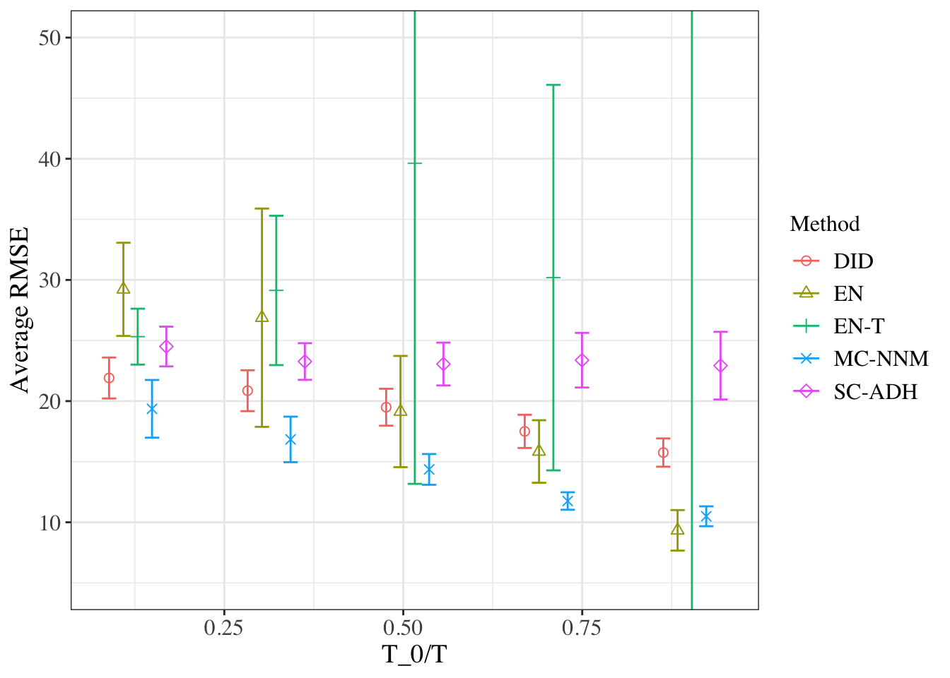

8.7 Further Reading

For interested readers, Athey, Bayati, Doudchenko, Imbens, and Khosravi (2021) contains more details on the topic.