Chapter 3 Risk Parity Portfolios

3.1 Introduction

The “risk parity” approach was popularized by Ray Dalio’s Bridgewater Associates - the largest hedge fund by assets under management ($132.8 billions of USD) - with the creation of the All Weather asset allocation strategy in 1996. “All Weather” is a term used to designate funds that tend to perform reasonably well during both favorable and unfavorable economic and market conditions. Today, several managers have employed “All Weather” concepts under a risk parity approach.

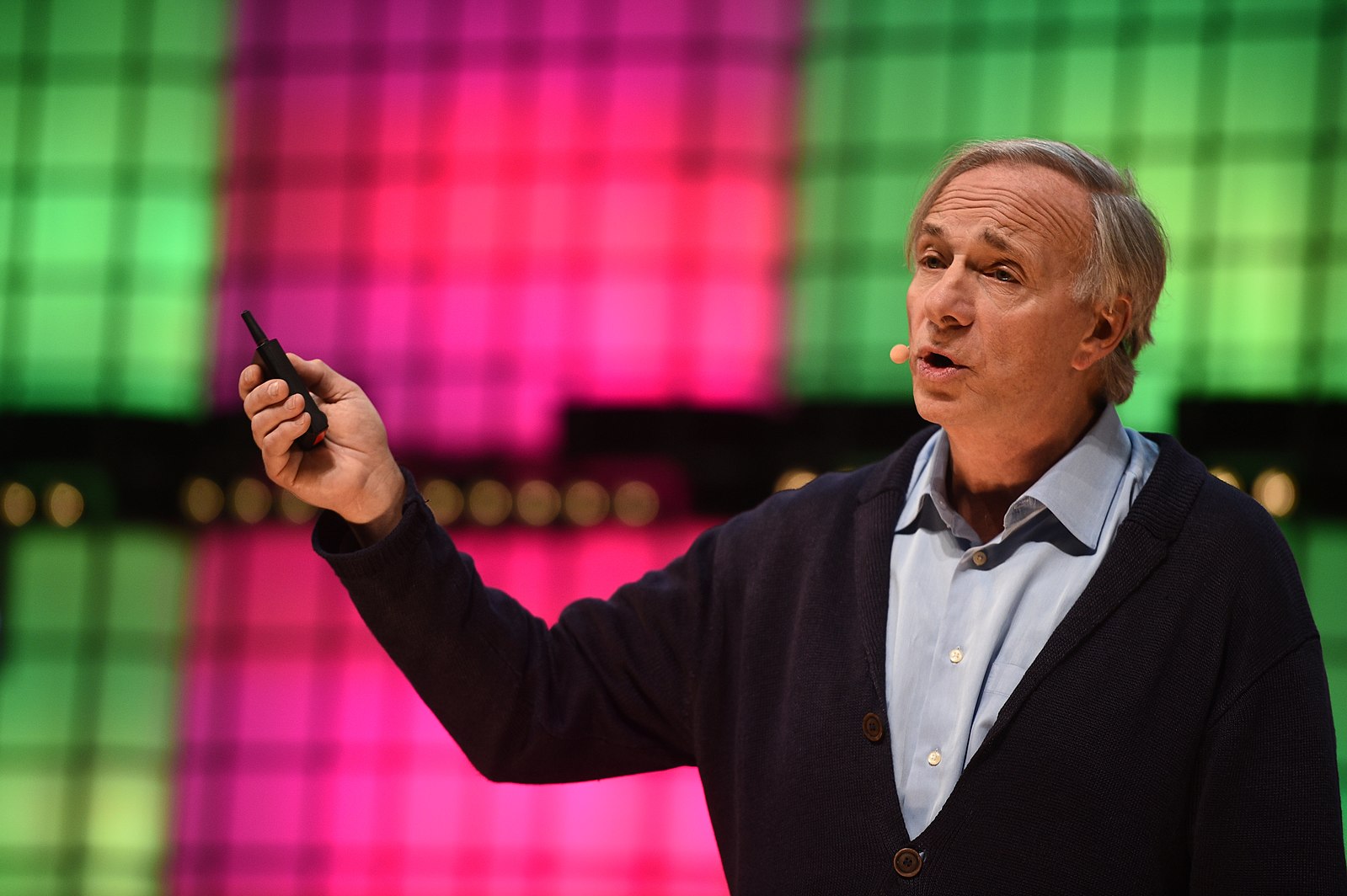
Figure 3.1: 7 November 2018; Ray Dalio, Bridgewater Associates on Centre Stage during day two of Web Summit 2018 at the Altice Arena in Lisbon, Portugal. Photo by David Fitzgerald/Web Summit via SportsfilePhoto by David Fitzgerald /Sportsfile.

A risk parity portfolio seeks to achieve an equal balance between the risk associated with each asset class or portfolio component. In that way, lower risk asset classes will generally have higher notional allocations than higher risk asset classes.

Risk Parity is about Balance - Bridgewater.

Risk parity strategies suffered in recent history (2010-2017) as the bull market has pushed stocks to a record high hence favoring equity-concentrated portfolios. However, the increase in market volatility since 2018, the emergency of geo-political and tradewars risk as well as the growth in haven assets like Gold create conditions that strengthen the case for diversified portfolios. This is demonstrated in Fig. 3.2 which shows that the S&P risk parity strategy has returned almost 10% over the last 12 months (Aug/2018 - Aug-2019), more than double the S&P 500 index of U.S. stocks.

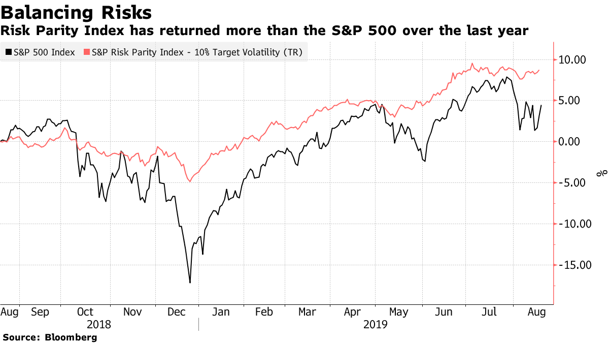
Figure 3.2: S&P 500 index versus S&P Risk Parity Index. Source: Bloomberg.

In Aug/2019, there have been news about the launch of a new Risk Parity ETF in the US. The RPAR Risk Parity ETF plans to allocate across asset classes based on risk, regulatory filings show. The fund would be the first in the U.S. to follow this quantitative approach, allotting more money to securities with lower volatility according to Bloomberg.

[The RPAR Risk Parity ETF is] kind of like Bridgewater does, but they just do it for the wealthiest institutions in the world. The idea here is to build something that would work for everybody. - Alex Shahidi, former relationship manager at Dalio’s Bridgewater Associate and creator of the RPAR Risk Parity ETF. Bloomberg.

But how can we a risk parity portfolio? How does it perform against a traditional mean/variance model?

In this Chapter,

1. We will show how you can build your own Risk Parity portfolio
2. We will create and compare the performance two indices:

• A FAANG Risk Parity Index of FAANG companies with equal risk balance
• A FAANG Tangency Portfolio Index of FAANG companies with weights such that return/risk ratio is maximized

By the end of the Chapter, you will be able to create your own risk parity / All Weather fund and compare it against your benchmark of choice.

3.2 Risk Parity Portfolio

A risk parity portfolio denotes a class of portfolios whose assets verify the following equalities (Vinicius and Palomar 2019): \[\begin{equation} w_{i} \frac{\partial f(\mathbf{w})}{\partial w_{i}}=w_{j} \frac{\partial f(\mathbf{w})}{\partial w_{j}}, \forall i, j \end{equation}\]

where \(f\) is a positively homogeneous function of degree one that measures the total risk of the portfolio and \(\mathbf{w}\) is the portfolio weight vector. In other words, the marginal risk contributions for every asset in a risk parity portfolio are equal. A common choice for \(f\), for instance, is the standard deviation of the portfolio, which is usually called volatility, i.e., \(f(\mathbf{w})=\sqrt{\mathbf{w}^{T} \mathbf{\Sigma} \mathbf{w}}\), where \(\mathbf{\Sigma}\) is the covariance matrix of assets.

In practice, risk and portfolio managers have risk mandates they follow or bounds for marginal risk contributions at the asset, country, regional or sector levels. Hence, a natural extension of the risk parity portfolio is the so called risk budget portfolio, in which the marginal risk contributions match preassigned quantities (Vinicius and Palomar 2019). Mathematically, \[\begin{equation} w_{i}(\Sigma \mathbf{w})_{i}=b_{i} \mathbf{w}^{T} \Sigma \mathbf{w}, \forall i, \end{equation}\]

where \(\mathbf{b} \triangleq\left(b_{1}, b_{2}, \ldots, b_{N}\right)\left(\text { with } \mathbf{1}^{T} \mathbf{b}=1 \text { and } \mathbf{b} \geq \mathbf{0}\right)\) is the vector of desired marginal risk contributions.

3.3 Tangency Portfolio

Mean variance optimization is a commonly used quantitative tool part of Modern Portfolio Theory that allows investors to perform allocation by considering the trade-off between risk and return.

Figure 3.3: In 1990, Dr. Harry M. Markowitz shared The Nobel Prize in Economics for his work on portfolio theory.

In a mean-variance framework, the objective is to minimize portfolio risk \(\sigma^2\) subject to a baseline expected rate of return \(\mu_b\) as follows: \[\begin{equation} \begin{array}{ll}{\mathcal{M}} & {\text { minimize } \quad \frac{1}{2} w^{T} \Sigma w} \\ {\text { subject to }} & {\mathrm{m}^{T} w \geq \mu_{b}, \text { and } \mathbf{1}^{T} w=1}\end{array} \end{equation}\]

where \(m\) is the vector of expected returns for the portfolio assets.

We will obtain an optimal portfolio (min risk) for each target rate of return \(\mu_b\) thus forming an efficient frontier. Each point in the efficient frontier in Fig. 3.4 is a portfolio with an optimal combination of securities that minimized risk given a level of risk (standard deviation). The dots below the efficient frontier are portfolios with inferior performance. They either offer the same returns but with higher risk, or they offer less return for the same risk.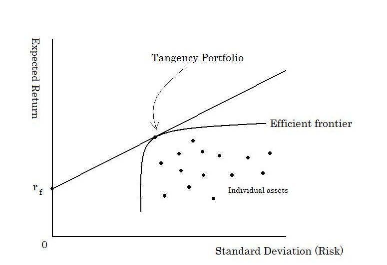

Figure 3.4: Efficienty Frontier. Attribution: ShuBraque (CC BY-SA 3.0)

But how can we choose a portfolio from the efficient frontier? One approach is to choose the most efficient portfolio from a risk/return standpoint, i.e., the portfolio with the highest Sharpe ratio (ratio between excess return and portfolio standard deviation). This portfolio is called the tangency portfolio and it’s located at the tangency point of the Capital Allocation Line and the Efficient Frontier.

We will implement both a parity risk and a tangency portfolio in the next section.

3.4 Optimizing FAANG: Ray Dalio versus Markowitz

3.4.1 Single Portfolio

First, we will load log-returns of adjusted prices for FAANG companies, i.e., the stocks identified by the following tickers: FB, AMZN, AAPL, NFLX and GOOG (see Appendix B.2 for code used to generate this dataset).

library(xts)
# load FAANG returns
faang.returns<-as.xts(read.zoo('./data/FAANG.csv',
                               header=TRUE,
                               index.column=1, sep=","))

We can use the packages riskParityPortfolio and fPortfolio to build a FAANG risk parity and tangency portfolios, respectively. We will first consider FAANG returns from 2018 to build the portfolios as follows:

library(IDPmisc)
library(riskParityPortfolio)
library(fPortfolio)

# consider returns from 2018
# omit days with missing data (INF/NA returns)
faang.returns.filtered <- NaRV.omit(as.matrix(faang.returns["2018"]))

# calculate covariance matrix
Sigma <- cov(faang.returns.filtered)

# compute risk parity portfolio
portfolio.parity <- riskParityPortfolio(Sigma)

# compute tangency portfolio
portfolio.tangency <- tangencyPortfolio(as.timeSeries(faang.returns.filtered), 
                                        constraints = "LongOnly")
portfolio.weights <- rbind(portfolio.parity$w, getWeights(portfolio.tangency))
row.names(portfolio.weights)<-c("Parity Portfolio", "Tangency Portfolio")

Fig. 3.5 shows the portfolio weights obtained for both the Parity and the Tangency portfolios. We observe that the Tangency portfolio concentrates the weights between Amazon and Netflix with both companies having nearly the same weight while Facebook, Apple and Google are left out of the portfolio. On the other hand, the Parity portfolio presents a well-balanced distribution of weights among the FAANG companies with all company weights around 20%. Apple and Google have weights a little over 20% while Netflix is the company with the lowest weight (15%).

barplot(portfolio.weights, main = "", xlab = "stocks", ylab = "dollars",
        beside = TRUE, legend = TRUE, col=c("black", "red"),
        args.legend = list(bg = "white"))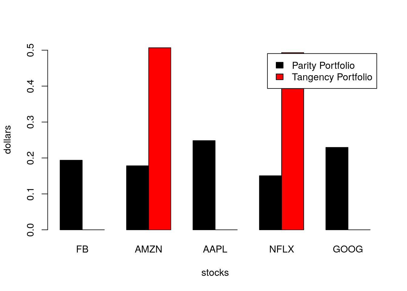

Figure 3.5: Portfolio weights for parity and tangency FAANG portfolios considering returns from 2018.

Fig. 3.6 compares the (covariance) risk budget of the Parity and Tangency portfolios obtained. As expected, we observe that the Parity portfolio has a risk budget equally distributed among the portfolio assets. On the other hand, the Tangency portfolio concentrates the risk between Amazon and Netflix with the latter corresponding to over 56% of the risk budget of the portfolio.

portfolio.risks <- rbind(portfolio.parity$risk_contribution/sum(portfolio.parity$risk_contribution), getCovRiskBudgets(portfolio.tangency))
row.names(portfolio.risks)<-c("Parity Portfolio", "Tangency Portfolio")
barplot(portfolio.risks, main = "", xlab = "stocks", ylab = "Covariance Risk Budget",
        beside = TRUE, legend = TRUE, col=c("black", "red"),
        args.legend = list(bg = "white"))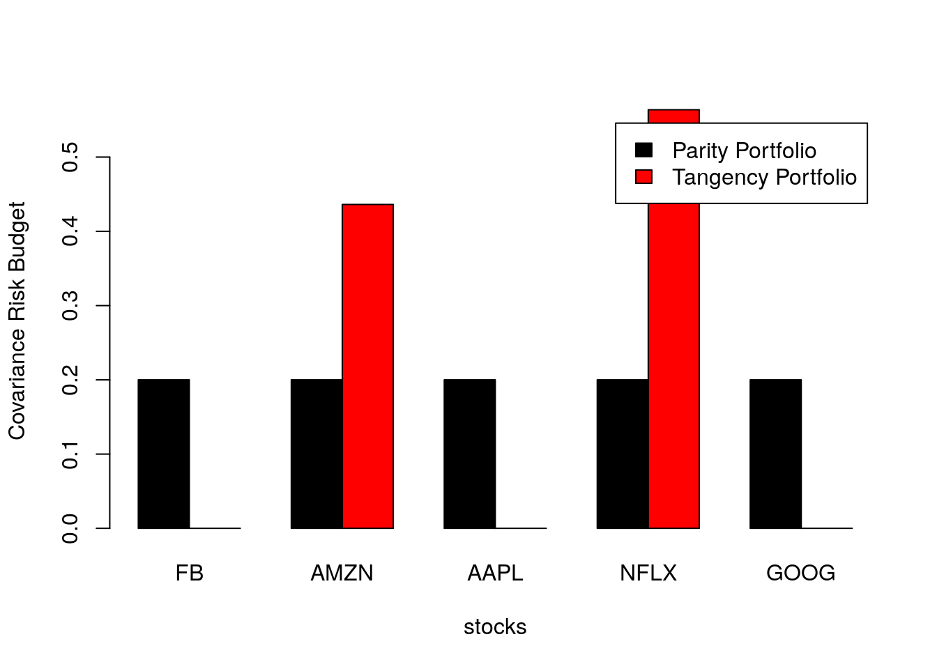

Figure 3.6: Portfolio covariance risk budget for parity and tangency FAANG portfolios considering returns from 2018.

3.4.2 The Ray Dalio FAANG Index

What would be the performance of a “Ray Dalio FAANG Index” i.e. a portfolio composed of FAANG companies and rebalanced to match a corresponding Risk Parity portfolio? Would it beat a corresponding Tagency portfolio?

To answer these questions, we will consider a portfolio of FAANG companies in the time period from 2014-01-01 and 2019-09-01 and build two indices:

1. Risk Parity Index: Rebalances portfolio weights quarterly setting the weights according to a risk parity portfolio;
2. Tangency Portfolio Index: Rebalances portfolio weights quarterly setting weights according to a Tangency portfolio.

We first define our rebalance dates by constructing a rolling window of 12-month width and a 3-month step-size as follows:

library(fPortfolio)
faang.returns.xts<-faang.returns["2014-01-01/2019-09-01"]
rWindows<-rollingWindows(faang.returns.xts, period="12m",
                         by="3m")

Our rebalance dates are the following:

print(rWindows$to)

## GMT
##  [1] [2014-12-31] [2015-03-31] [2015-06-30] [2015-09-30] [2015-12-31]
##  [6] [2016-03-31] [2016-06-30] [2016-09-30] [2016-12-31] [2017-03-31]
## [11] [2017-06-30] [2017-09-30] [2017-12-31] [2018-03-31] [2018-06-30]
## [16] [2018-09-30] [2018-12-31] [2019-03-31] [2019-06-30]

Next, we calculate risk parity portfolio weights at each rebalance date considering returns in a 12-month window as follows:

# Apply FUN to time-series R in the subset [from, to].
ApplyFilter <- function(from, to, R, FUN){
  return(FUN(R[paste0(from, "/", to)]))
}
# For each pair (from, to) ApplyFilter to time-series R using FUN
ApplyRolling <- function(from, to, R, FUN){
  library(purrr)
  return(map2(from, to, ApplyFilter, R=R, FUN=FUN))
}
# Returns weights of a risk parity portfolio from covariance matrix of matrix of returns r
CalculateRiskParity <- function(r){
  library(riskParityPortfolio)
  return(riskParityPortfolio(cov(r))$w)
}
# Given a matrix of returns `r`,
# calculates risk parity weights for each date in `to` considering a time window from `from` and `to` 
RollingRiskParity <- function(from, to, r){
  library(rlist)
  p<-ApplyRolling(from, to, r, CalculateRiskParity)
  names(p)<-to
  return(list.rbind(p))
}

parity.weights<-RollingRiskParity(rWindows$from@Data, rWindows$to@Data, faang.returns.xts)

We now calculate quarterly weights for FAANG tangency portfolios. We leverage the fPortfolio package to calculate a rolling tangency portfolio as follows:

library(fPortfolio)
faang.returns.ts<-as.timeSeries(faang.returns.xts)
Spec = portfolioSpec()

rolling.portfolio.tangency <- rollingTangencyPortfolio(faang.returns.ts,
                                                       constraints = "LongOnly",
                                                       from=rWindows$from,
                                                       to=rWindows$to,
                                                       spec=Spec)

names(rolling.portfolio.tangency)<-rWindows$to
tan.weights <- sapply(rolling.portfolio.tangency,getWeights)
rownames(tan.weights) <- colnames(faang.returns.ts)
tan.weights<-t(tan.weights)

Figs. 3.7 and 3.8 show the portfolio weights obtained for parity risk and tangency portfolios, respectively. We observe that the risk parity weights are quite stable over time with Netflix having a slightly underweighting compared to the other portfolio constituents. On the other hand, the tangency portfolio weights vary considerably throughout the time period considered, which can impose challenges in its maintenance as its turnover can be quite high. The tangency portfolio overweights Apple and Amazon across many rebalance dates and it underweights Google in all rebalance dates.

PerformanceAnalytics::chart.StackedBar(parity.weights, 
                 xlab = "Rebalance Dates",
                 ylab = "Weight", 
                 main = "FAANG Risk Parity")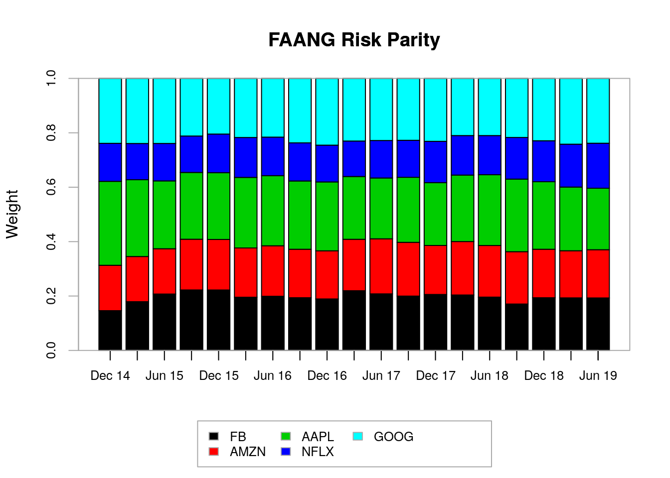

Figure 3.7: Portfolio weights for FAANG risk parity portfolios.

PerformanceAnalytics::chart.StackedBar(tan.weights, xlab = "Rebalance Dates",
                 ylab = "Weight", 
                 main = "FAANG Tangency Portfolio")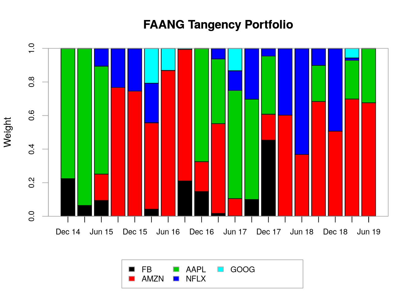

Figure 3.8: Portfolio weights for FAANG tangency portfolios.

We will use the time series of FAANG companies and the time series of risk parity and tangency portfolio weights to calculate the returns of the risk parity and tangency portfolio indexes as follows:

library(PerformanceAnalytics)
tan.returns <- Return.portfolio(faang.returns.xts, weights=tan.weights,verbose=TRUE)
parity.returns <- Return.portfolio(faang.returns.xts, weights=parity.weights,verbose=TRUE)
p.returns<-merge(tan.returns$returns, parity.returns$returns)
names(p.returns)<-c("FAANG Tangency Index", "FAANG Parity Index")

Fig. 3.9 shows the performance summary for the risk parity index versus the tangency portfolio index. Surprisingly, the FAANG risk parity index outperforms the FAANG tangency portfolio index by quite a bit with a cumulative return of 169.482% versus 109.652% from the tangency portfolio index. The FAANG risk parity index also has a relatively lower drawdown across most of the period analyzed.

### Performance Summary (return / drawdown)
PerformanceAnalytics::charts.PerformanceSummary(p.returns, colorset=rich6equal,
                          lwd=2, cex.legend = 1.0, event.labels = TRUE, main = "")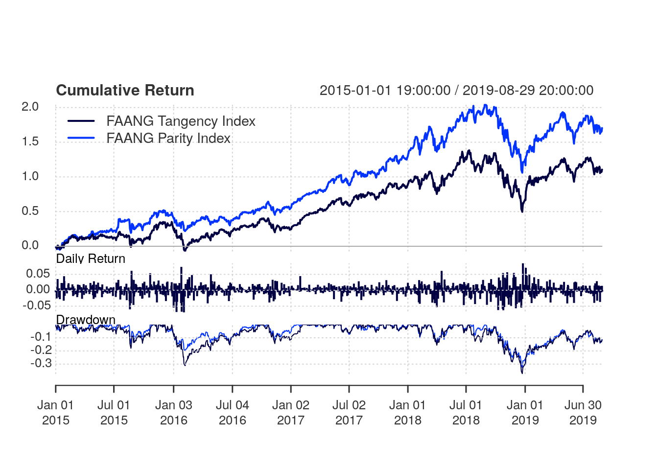

Figure 3.9: Performance summary for the risk parity index versus the tangency portfolio index

Tables 3.1 and 3.2 show the calendar returns for the risk parity and tangency portfolio indexes, respectively. Interestingly, in years where the tangency portfolio index had positive cumulative return, the risk parity index yielded less returns than the tangency portfolio index. Conversely, in years where the tangency portfolio index had negative cumulative return, the risk parity index showed superior performance than the tangency portfolio index. In that way, the risk parity index showed “not as good” but also “not as bad” yearly returns compared to the tangency portfolios.

Table 3.1: Calendar Returns (%): FAANG Parity Index

	2015	2016	2017	2018	2019
Jan	2.1	0.6	2.1	-0.6	-1.2
Feb	-1.1	3.7	1.4	-1.6	1.0
Mar	-0.6	1.3	0.0	2.3	1.6
Apr	0.9	1.7	1.7	1.4	0.9
May	0.4	-0.6	0.1	1.8	-2.2
Jun	0.6	1.3	-0.4	-0.4	1.3
Jul	-0.4	1.3	0.5	1.8	-1.1
Aug	-4.2	0.2	-0.1	-0.2	-0.4
Sep	0.9	0.7	0.8	0.3	NA
Oct	-0.7	-1.0	0.2	1.7	NA
Nov	1.8	-1.2	-0.9	0.3	NA
Dec	-1.8	-1.3	-0.8	0.8	NA
FAANG Parity Index	-2.1	6.9	4.6	7.8	0.0

Table 3.2: Calendar Returns (%): FAANG Tangency Index

	2015	2016	2017	2018	2019
Jan	-1.7	-1.0	4.5	0.6	-2.6
Feb	-1.6	4.8	1.7	-1.4	0.8
Mar	-0.3	1.5	0.0	2.4	2.4
Apr	2.8	5.0	2.3	0.7	0.5
May	0.3	-0.5	0.2	1.4	-2.1
Jun	1.0	2.1	-0.4	-0.5	1.6
Jul	-0.4	1.1	0.7	0.6	-1.2
Aug	-4.6	0.2	0.0	-0.3	-0.4
Sep	0.4	0.9	0.6	1.1	NA
Oct	0.5	-0.7	-0.4	3.6	NA
Nov	2.0	-1.3	-0.5	0.5	NA
Dec	-1.9	-1.8	-0.9	1.7	NA
FAANG Tangency Index	-3.7	10.3	7.9	11.0	-1.2

Fig. 3.10 shows the performance summary in a rolling 252-day window. Again, we observe that the risk parity index presents a superior performance compared to the tangency portfolio index. The risk parity index presents higher annualized return, lower standard deviation and superior Sharpe ratio in most of the period analyzed compared to the tangency portfolio index. As presented in Tab. 3.3, the risk parity index has a total of 23.71% annualized return, 22.55% standard deviation and 1.051 Sharpe-ratio versus 17.22% annualized return, 26.42% standard deviation and 0.652 Sharpe-ratio from the tangency portfolio index.

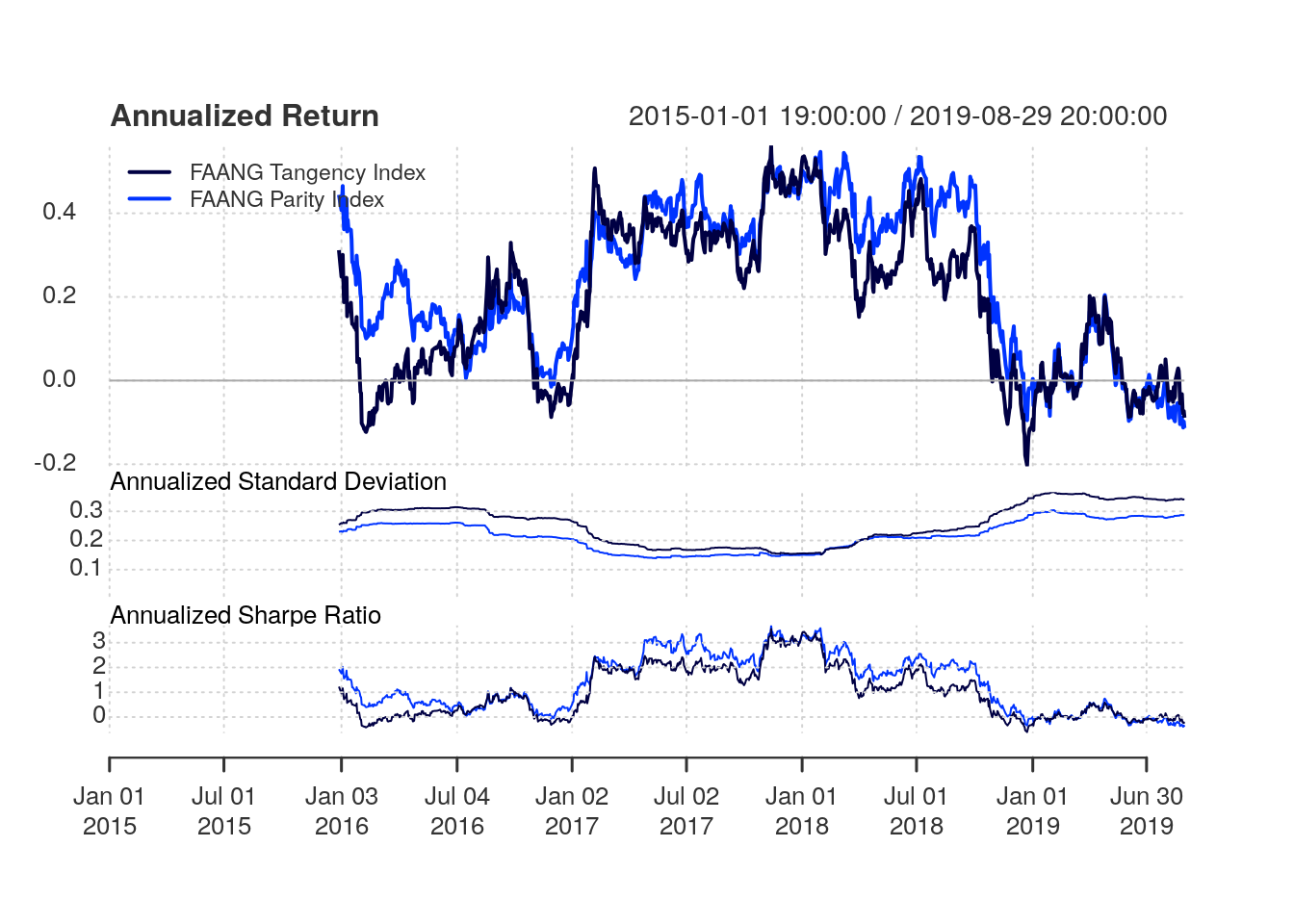
Figure 3.10: Performance summary in a rolling 252-day window for the risk parity index versus the tangency portfolio index

Table 3.3: Annualized Returns

	FAANG Tangency Index	FAANG Parity Index
Annualized Return	0.172	0.237
Annualized Std Dev	0.264	0.226
Annualized Sharpe (Rf=0%)	0.652	1.051

3.5 Discussion and Conclusion

What mix of assets has the best chance of delivering good returns over time through all economic environments?

That was the question posed by Bridgewater Associates before creating the All Weather funds with concepts today popularized in the so-called risk parity strategies.

The traditional approach to asset allocation often tolerates higher concentration of risk with the objective to generate higher longer-term returns. Bridgewater argues that this approach has a serious flaw:

If the source of short-term risk is a heavy concentration in a single type of asset, this approach brings with it a significant risk of poor long-term returns that threatens the ability to meet future obligations. This is because every asset is susceptible to poor performance that can last for a decade or more, caused by a sustained shift in the economic environment - Bridgewater.

In this Chapter, we introduced the concept of risk parity portfolios and compare it against a mean-variance model. We provided a simple practical example by constructing a FAANG risk parity index and comparing its performance against a FAANG tangency index, which selects the portfolio from the mean-variance efficient frontier with optimal Sharpe-ratio.

The risk parity index presented higher annualized return, lower standard deviation and superior Sharpe ratio in most of the period analyzed compared to the tangency portfolio index. Of course, results should be taken with caution.

In practice, both the risk parity and mean-variance approaches are employed in larger portfolios potentially across multiple asset classes. Those methodologies strive when there are assets that are uncorrelated in the portfolio which can increase the potential for diversification. Further, modern portfolio optimization strategies can be much more complex with a variety of objective functions and constraints. Our objective in this article was to give you a head start. Feel free to check out the source code in our github project and implement your own strategies!