Chapter 5 How to Measure Statistical Causality: A Transfer Entropy Approach with Financial Applications
We’ve all heard the say “correlation does not imply causation”, but how can we quantify causation? This is an extremely difficult and often misleading task, particularly when trying to infer causality from observational data and we cannot perform controlled trials or A/B testing.
Take for example the 2-dimensional system from Fig. 5.1.
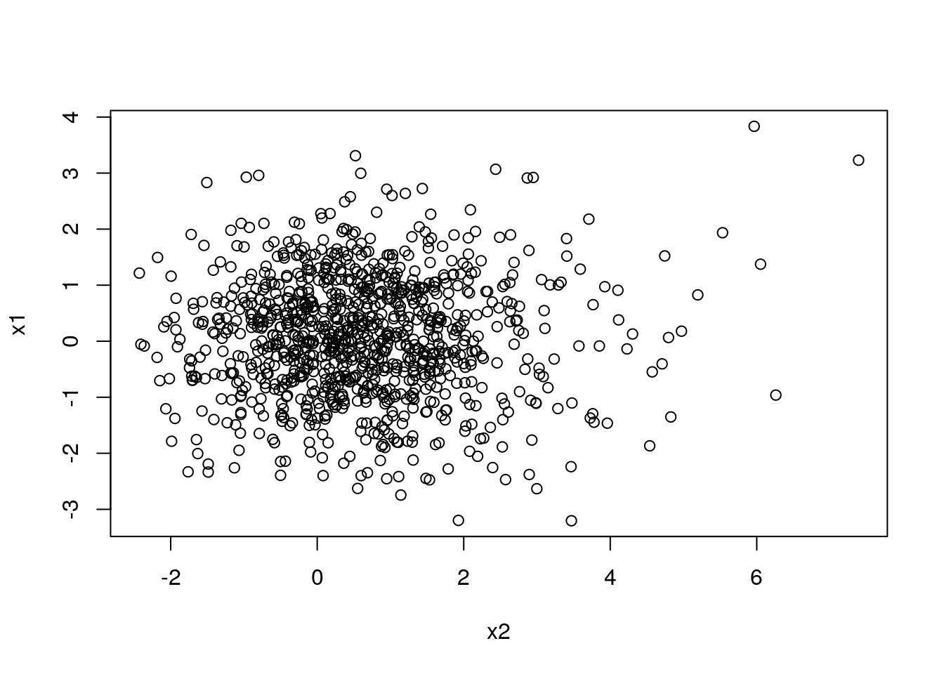
Figure 5.1: Life is Random (or Nonlinear?)
A simple nonlinearity introduced in the relationship between \(x_2\) and \(x_1\) was enough to introduce complexity into the system and potentially mislead a naive (non-quant) human.
Fortunately, we can take advantage of statistics and information theory to uncover complex causal relationships from observational data (remember, this is still a very challenging task).
The objectives of this Chapter are the following:
- Introduce a prediction-based definition of causality and its implementation using a vector auto-regression formulation.
- Introduce a probabilistic-definition of causality and its implementation using an information-theoretical framework.
- Simulate linear and nonlinear systems and uncover causal links with the proposed methods.
- Quantify information flow among global equity indexes further uncovering which indexes are driving the global financial markets.
- Discuss further applications including the impact of social media sentiment in financial and crypto markets.
5.1 A First Definition of Causality
We quantify causality by using the notion of the causal relation introduced by Granger (Wiener 1956; Granger 1969), where a signal \(X\) is said to Granger-cause \(Y\) if the future realizations of \(Y\) can be better explained using the past information from \(X\) and \(Y\) rather than \(Y\) alone.

Figure 5.2: Economist Clive Granger, who won the 2003 Nobel Prize in Economics.
The most common definitions of Granger-causality (G-causality) rely on the prediction of a future value of the variable \(Y\) by using the past values of \(X\) and \(Y\) itself. In that form, \(X\) is said to G-cause \(Y\) if the use of \(X\) improves the prediction of \(Y\).
Let \(X_t\) be a random variable associated at time \(t\) while \(X^t\) represents the collection of random variables up to time \(t\). We consider \({X_t}, {Y_t}\) and \({Z_t}\) to be three stochastic processes. Let \(\hat Y_{t+1}\) be a predictor for the value of the variable \(Y\) at time \(t+1\).
We compare the expected value of a loss function \(g(e)\) with the error \(e=\hat{Y}_{t+1} - Y_{t+1}\) of two models:
- The expected value of the prediction error given only \(Y^t\) \[\begin{equation} \mathcal{R}(Y^{t+1} \, | \, Y^t,Z^t) = \mathbb{E}[g(Y_{t+1} - f_1(X^{t},Z^t))] \end{equation}\]
- The expected value of the prediction error given \(Y^t\) and \(X^t\) \[\begin{equation} \mathcal{R}(Y^{t+1} \, | \, X^{t},Y^t,Z^t) = \mathbb{E}[g(Y_{t+1} - f_2(X^{t},Y^t,Z^t))]. \end{equation}\]
In both models, the functions \(f_1(.)\) and \(f_2(.)\) are chosen to minimize the expected value of the loss function. In most cases, these functions are retrieved with linear and, possibly, with nonlinear regressions, neural networks etc. Typical forms for \(g(.)\) are the \(l1\)- or \(l2\)-norms.
We can now provide our first definition of statistical causality under the Granger causal notion as follows:
Standard Granger-causality tests assume a functional form in the relationship among the causes and effects and are implemented by fitting autoregressive models (Wiener 1956; Granger 1969).
Consider the linear vector-autoregressive (VAR) equations: \[\begin{align} Y(t) &= {\alpha} + \sum^k_{\Delta t=1}{{\beta}_{\Delta t} Y(t-\Delta t)} + \epsilon_t, \tag{5.1}\\ Y(t) &= \widehat{\alpha} + \sum^k_{\Delta t=1}{{\widehat{\beta}}_{\Delta t} Y(t-\Delta t)} + \sum^k_{\Delta t=1}{{\widehat{\gamma}}_{\Delta t}X(t-\Delta t)}+ \widehat{\epsilon}_t, \tag{5.2} \end{align}\]where \(k\) is the number of lags considered. Alternatively, you can choose your DL/SVM/RF/GLM method of choice to fit the model.
From Def. 5.1, \(X\) does not G-cause \(Y\) if and only if the prediction errors of \(X\) in the restricted Eq. (5.1) and unrestricted regression models Eq. (5.2) are equal (i.e., they are statistically indistinguishable). A one-way ANOVA test can be utilized to test if the residuals from Eqs. (5.1) and (5.2) differ from each other significantly. When more than one lag \(k\) is tested, a correction for multiple hypotheses testing should be applied, e.g. False Discovery Rate (FDR) or Bonferroni correction.
5.2 A Probabilistic-Based Definition
A more general definition than Def. 5.1 that does not depend on assuming prediction functions can be formulated by considering conditional probabilities. A probabilistic definition of G-causality assumes that \(Y_{t+1}\) and \(X^{t}\) are independent given the past information \((X^{t}, Y^{t})\) if and only if \(p(Y_{t+1} \, | \, X^{t}, Y^{t}, Z^{t}) = p(Y_{t+1} \, | \, Y^{t}, Z^{t})\), where \(p(. \, | \, .)\) represents the conditional probability distribution. In other words, omitting past information from \(X\) does not change the probability distribution of \(Y\). This leads to our second definition of statistical causality as follows:
Def. 5.2 does not assume any functional form in the coupling between \(X\) and \(Y\). Nevertheless, it requires a method to assess their conditional dependency. In the next section, we will leverage an Information-Theoretical framework for that purpose.
5.3 Transfer Entropy and Statistical Causality
Given a coupled system \((X,Y)\), where \(P_Y(y)\) is the pdf of the random variable \(Y\) and \(P_{X,Y}\) is the joint pdf between \(X\) and \(Y\), the joint entropy between \(X\) and \(Y\) is given by the following: \[\begin{equation} H(X,Y) = -\sum_{x \in X}{\sum_{y \in Y}{P_{X,Y}(x,y)\log{P_{X,Y}(x,y)}}}. \label{eq:HXY} \end{equation}\] The conditional entropy is defined by the following: \[\begin{equation} H\left(Y\middle\vert X\right) = H(X,Y) - H(X). \end{equation}\]We can interpret \(H\left(Y\middle\vert X\right)\) as the uncertainty of \(Y\) given a realization of \(X\).

Figure 5.3: Shannon, Claude. The concept of information entropy was introduced by Claude Shannon in his 1948 paper: A Mathematical Theory of Communication.
To compute G-Causality, we use the concept of Transfer Entropy. Since its introduction (Schreiber 2000), Transfer Entropy has been recognized as an important tool in the analysis of causal relationships in nonlinear systems (Hlavackovaschindler et al. 2007). It detects directional and dynamical information (Montalto 2014) while not assuming any particular functional form to describe interactions among systems.
The Transfer Entropy can be defined as the difference between the conditional entropies: \[\begin{equation} TE\left(X \rightarrow Y\right \vert Z) = H\left(Y^F\middle\vert Y^P,Z^P\right) - H\left(Y^F\middle\vert X^P, Y^P,Z^P\right), \tag{5.3} \end{equation}\] which can be rewritten as a sum of Shannon entropies: \[\begin{align} TE\left(X \rightarrow Y\right) = H\left(Y^P, X^P\right) - H\left(Y^F, Y^P, X^P\right) + H\left(Y^F, Y^P\right) - H\left(Y^P\right), \end{align}\]where \(Y^F\) is a forward time-shifted version of \(Y\) at lag \(\Delta t\) relatively to the past time-series \(X^P\), \(Y^P\) and \(Z^P\). Within this framework we say that \(X\) does not G-cause \(Y\) relative to side information \(Z\) if and only if \(H\left(Y^F\middle\vert Y^P,Z^P \right) = H\left(Y^F\middle\vert X^P, Y^P,Z^P\right)\), i.e., when \(TE\left(X \rightarrow Y,Z^P\right) = 0\).
5.4 Net Information Flow
Transfer-entropy is an asymmetric measure, i.e., \(T_{X \rightarrow Y} \neq T_{Y \rightarrow X}\), and it thus allows the quantification of the directional coupling between systems. The Net Information Flow is defined as \[\begin{equation} \widehat{TE}_{X \rightarrow Y} = TE_{X \rightarrow Y} - TE_{Y \rightarrow X}\;. \end{equation}\]One can interpret this quantity as a measure of the dominant direction of the information flow. In other words, a positive result indicates a dominant information flow from \(X\) to \(Y\) compared to the other direction or, similarly, it indicates which system provides more predictive information about the other system (Michalowicz, Nichols, and Bucholtz 2013).
5.5 The Link Between Granger-causality and Transfer Entropy
It has been shown (Barnett, Barrett, and Seth 2009) that linear G-causality and Transfer Entropy are equivalent if all processes are jointly Gaussian. In particular, by assuming the standard measure (\(l2\)-norm loss function) of linear G-causality for the bivariate case as follows (see Section 5.1 for more details on linear-Granger causality):
\[\begin{equation} GC_{X \rightarrow Y} = \log\left( \frac{var(\epsilon_t)}{var( \widehat{\epsilon}_t)} \right), \tag{5.4} \end{equation}\]the following can be proved (Barnett, Barrett, and Seth 2009):
\[\begin{align} TE_{X \rightarrow Y} = GC_{X \rightarrow Y}/2. \tag{5.5} \end{align}\]This result provides a direct mapping between the Transfer Entropy and the linear G-causality implemented in the standard VAR framework. Hence, it is possible to estimate the TE both in its general form and with its equivalent form for linear G-causality.
5.6 Information Flow on Simulated Systems
In this section, we construct simulated systems to couple random variables in a causal manner. We then quantify information flow using the methods studied in this Chapter.
We first assume a linear system, where random variables have linear relationships defined as follow: \[\begin{align} x_1(n) &= 0.95\sqrt{2}x_1(n-1) - 0.9025x_1(n-1) + w_1\\ \nonumber x_2(n) &= 0.5x_1(n-1) + w_2\\ \nonumber x_3(n) &= -0.4x_1(n-1) + w_3\\ \nonumber x_4(n) &= -0.5x_1(n-1) + 0.25\sqrt{2}x_4(n-1) + 0.25\sqrt{2}x_5(n-1) + w_4\\ \nonumber x_5(n) &= -0.25\sqrt{2}x_4(n-1) + 0.25\sqrt{2}x_5(n-1) + w_5, \nonumber \end{align}\]where \(w_1, w_2, w_3, w_4, w_5 \sim N(0, 1)\). To simulate this system we assume \(x_i(0) = 0, i \in (1, 2, \ldots, 5)\) as initial condition and then iteratively generate \(x_i\) for \(n \in (1, 2, \ldots, N)\) with a total of \(N = 10,000\) iterations by randomly sampling \(w_i, i \in (1, 2, \ldots, 5)\) from a normal distribution with zero mean and unit variance.
We simulate this linear system with the following code:
set.seed(123)
n <- 10000
x1 <- x2<-x3<-x4<-x5<-rep(0, n + 1)

for (i in 2:(n + 1)) {
  x1[i] <- 0.95 * sqrt(2)* x1[i - 1] -0.9025*x1[i - 1] + rnorm(1, mean=0, sd=1)
  x2[i] <- 0.5*x1[i - 1] + rnorm(1, mean=0, sd=1)
  x3[i] <- -0.4*x1[i - 1] + rnorm(1, mean=0, sd=1)
  x4[i] <- -0.5*x1[i - 1] + 0.25*sqrt(2)*x4[i - 1] + 0.25*sqrt(2)*x5[i - 1] + rnorm(1, mean=0, sd=1)
  x5[i] <- -0.25*sqrt(2)*x4[i - 1] + 0.25*sqrt(2)*x5[i - 1] + rnorm(1, mean=0, sd=1)
}

x1 <- x1[-1]
x2 <- x2[-1]
x3 <- x3[-1]
x4 <- x4[-1]
x5 <- x5[-1]
linear.system <- data.frame(x1, x2, x3, x4, x5)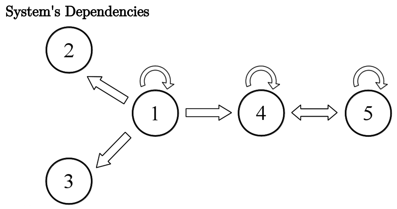
Figure 5.4: Interactions between the variables of the simulated linear system.
We first define a function that calculates a bi-variate measure for G-causality as defined in Eq. (5.4) as follows:
Linear.GC <- function(X, Y){

  n<-length(X)
  X.now<-X[1:(n-1)]
  Y.now<-Y[1:(n-1)]
  Y.fut<-Y[2:n]

  regression.uni=lm(Y.fut~Y.now)
  regression.mult=lm(Y.fut~Y.now+ X.now)
  var.eps.uni <- (summary(regression.uni)$sigma)^2
  var.eps.mult <- (summary(regression.mult)$sigma)^2
  GC <- log(var.eps.uni/var.eps.mult)
  return(GC)

}
We use the function calc_te from the package RTransferEntropy (Behrendt et al. 2019) and the previously defined function Linear.GC to calculate pairwise information flow among the simulated variables as follows:
library(RTransferEntropy)
library(future)

## Allow for parallel computing
plan(multiprocess)
## Warning: [ONE-TIME WARNING] Forked processing ('multicore') is disabled
## in future (>= 1.13.0) when running R from RStudio, because it is
## considered unstable. Because of this, plan("multicore") will fall
## back to plan("sequential"), and plan("multiprocess") will fall back to
## plan("multisession") - not plan("multicore") as in the past. For more
## details, how to control forked processing or not, and how to silence this
## warning in future R sessions, see ?future::supportsMulticore## Calculates GC and TE
GC.matrix<-FApply.Pairwise(linear.system, Linear.GC)
TE.matrix<-FApply.Pairwise(linear.system, calc_te)
rownames(TE.matrix)<-colnames(TE.matrix)<-var.names<-c("x1", "x2", "x3", "x4", "x5")
rownames(GC.matrix)<-colnames(GC.matrix)<-var.names
## Back to sequential
plan(sequential)The function FApply.Pairwise is an auxiliary function that simply applies a given function D.Func to all possible pairs of columns from a given matrix X as follows:
FApply.Pairwise <- function(X, D.Func){
  n = seq_len(ncol(X))

  ff.TE.value = function(a, b) D.Func(X[,a], X[,b])

  return(outer(n, n, Vectorize(ff.TE.value)))
}
Fig. 5.5 and Fig. 5.6 show Granger-causality and Transfer Entropy among the system’s variables, respectively. A cell \((x, y)\) presents the information flow from variable \(y\) to variable \(x\). We observe that both the Granger-causality (linear) and Transfer Entropy (nonlinear) approaches presented similar results, i.e., both methods captured the system’s dependencies similarly. This result is expected as the system is purely linear and Transfer Entropy is able to capture both the linear and nonlinear interactions.
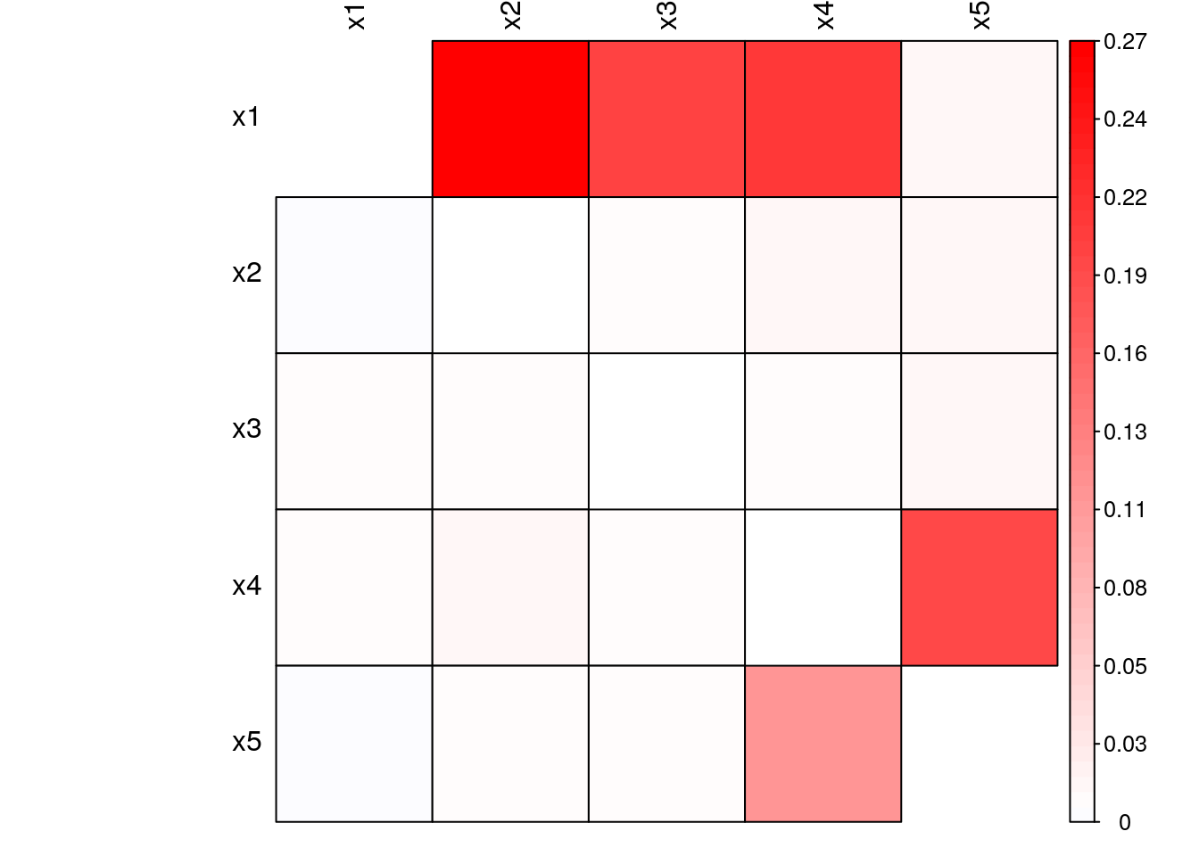
Figure 5.5: Granger-Causality of simulated linear system
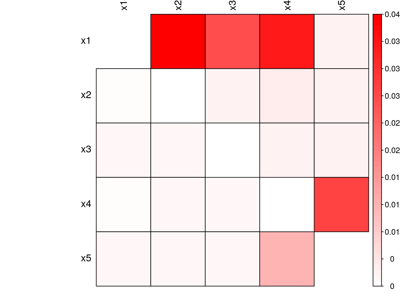
Figure 5.6: Transfer Entropy of simulated linear system
We define a second system by introducing nonlinear interactions between \(x_1\) and the variables \(x_2\) and \(x_5\) as follows:
\[\begin{align} x_1(n) &= 0.95\sqrt{2}x_1(n-1) - 0.9025x_1(n-1) + w_1\\ \nonumber x_2(n) &= 0.5x_1^2(n-1) + w_2\\ \nonumber x_3(n) &= -0.4x_1(n-1) + w_3\\ \nonumber x_4(n) &= -0.5x_1^2(n-1) + 0.25\sqrt{2}x_4(n-1) + 0.25\sqrt{2}x_5(n-1) + w_4\\ \nonumber x_5(n) &= -0.25\sqrt{2}x_4(n-1) + 0.25\sqrt{2}x_5(n-1) + w_5, \nonumber \end{align}\]where \(w_1, w_2, w_3, w_4\) and \(w_5 \sim N(0, 1)\). To simulate this system we assume \(x_i(0) = 0, i \in (1, 2, ..., 5)\) as initial condition and then iteratively generate \(x_i\) for \(n \in (1, 2, ..., N)\) with a total of \(N = 10,000\) iterations by randomly sampling \(w_i, i \in (1, 2, ..., 5)\) from a normal distribution with zero mean and unit variance.
We simulate this nonlinear system with the following code:
set.seed(123)
n <- 10000
x1 <- x2<-x3<-x4<-x5<-rep(0, n + 1)

for (i in 2:(n + 1)) {
  x1[i] <- 0.95 * sqrt(2)* x1[i - 1] -0.9025*x1[i - 1] + rnorm(1, mean=0, sd=1)
  x2[i] <- 0.5*x1[i - 1]^2 + rnorm(1, mean=0, sd=1)
  x3[i] <- -0.4*x1[i - 1] + rnorm(1, mean=0, sd=1)
  x4[i] <- -0.5*x1[i - 1]^2 + 0.25*sqrt(2)*x4[i - 1] + 0.25*sqrt(2)*x5[i - 1] + rnorm(1, mean=0, sd=1)
  x5[i] <- -0.25*sqrt(2)*x4[i - 1] + 0.25*sqrt(2)*x5[i - 1] + rnorm(1, mean=0, sd=1)
}

x1 <- x1[-1]
x2 <- x2[-1]
x3 <- x3[-1]
x4 <- x4[-1]
x5 <- x5[-1]
nonlinear.system <- data.frame(x1, x2, x3, x4, x5)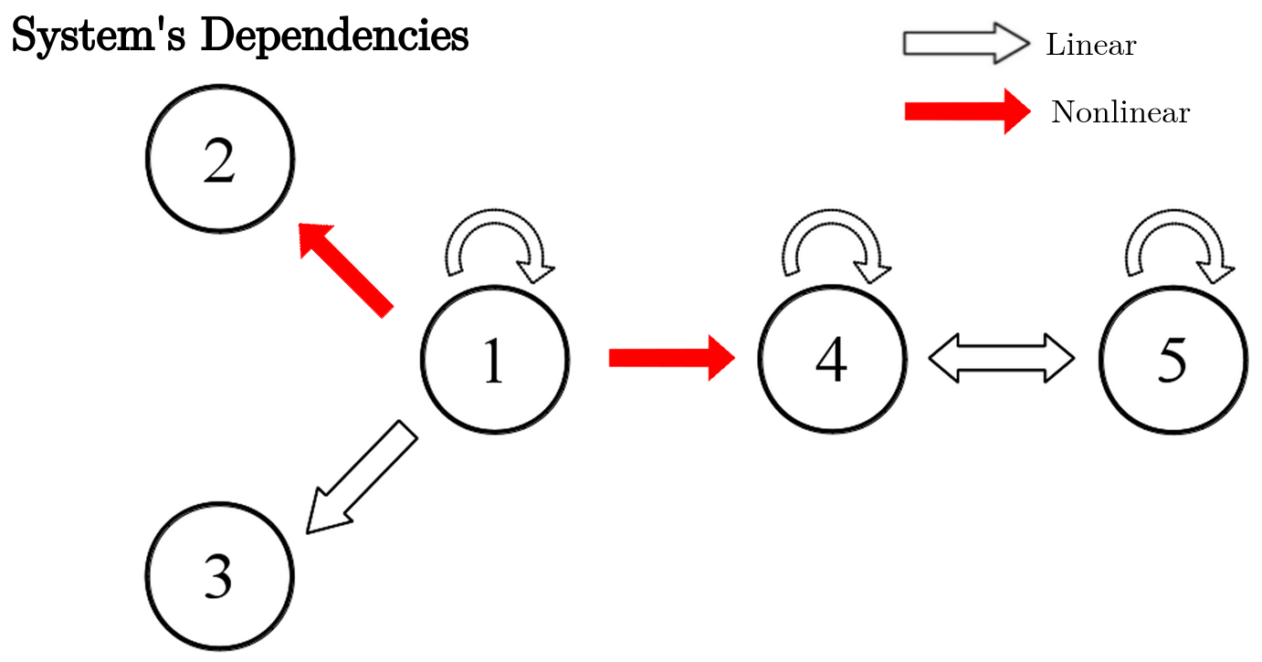
Figure 5.7: Interactions between the variables of the simulated nonlinear system.
We calculate Granger-causality and Transfer Entropy of the simulated nonlinear system as follows:
## Allow for parallel computing
plan(multiprocess)


## Calculates GC and TE
GC.matrix.nonlinear<-FApply.Pairwise(nonlinear.system, Linear.GC)
TE.matrix.nonlinear<-FApply.Pairwise(nonlinear.system, calc_te)

rownames(TE.matrix.nonlinear)<-colnames(TE.matrix.nonlinear)<-var.names
rownames(GC.matrix.nonlinear)<-colnames(GC.matrix.nonlinear)<-var.names

## Back to sequential computing
plan(sequential)
From Fig. 5.8 and Fig. 5.9, we observe that the nonlinear interactions introduced were not captured by the linear form of the information flow. While all linear interactions presented similar linear and nonlinear information flows, the two nonlinear interactions introduced in the system presented relatively higher nonlinear information flow compared to the linear formulation.
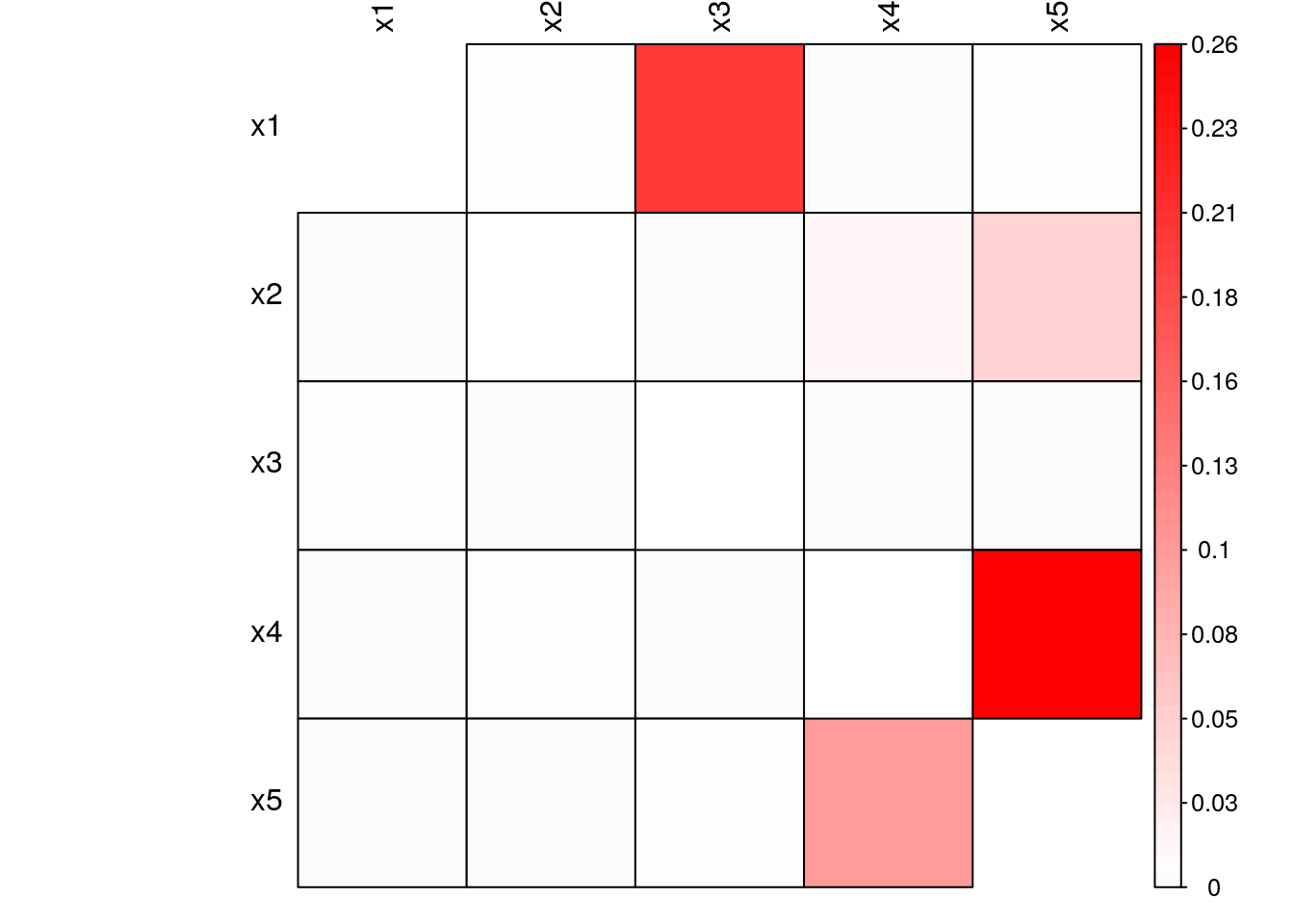
Figure 5.8: Granger-Causality of simulated nonlinear system
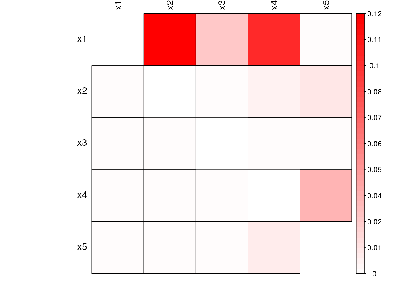
Figure 5.9: Transfer Entropy of simulated nonlinear system
5.7 Information Flow among International Stock Market Indices
The world’s financial markets form a complex, dynamic network in which individual markets interact with one another. This multitude of interactions can lead to highly significant and unexpected effects, and it is vital to understand precisely how various markets around the world influence one another (Junior, Mullokandov, and Kenett 2015).
In this section, we use Transfer Entropy for the identification of dependency relations among international stock market indices. First, we select some of the major global indices for our analysis, namely the S&P 500, the FTSE 100, the DAX, the EURONEXT 100 and the IBOVESPA, which track the following markets, respectively, the US, the UK, Germany, Europe and Brazil. They are defined by the following tickers:
tickers<-c("^GSPC", "^FTSE", "^GDAXI", "^N100", "^BVSP")Next, we will load log-returns of daily closing adjusted prices for the selected indices as follows (see Appendix B.1 for code used to generate this dataset):
library(xts)
dataset<-as.xts(read.zoo('./data/global_indices_returns.csv',
                  header=TRUE,
                  index.column=1, sep=","))
head(dataset)
## X.GSPC X.FTSE X.GDAXI X.N100 X.BVSP
## 2000-01-02 19:00:00 0.000000 NA 0.00000 0.00000 0.00000
## 2000-01-03 19:00:00 -0.039099 0.00000 -0.02456 -0.04179 -0.06585
## 2000-01-04 19:00:00 0.001920 -0.01969 -0.01297 -0.02726 0.02455
## 2000-01-05 19:00:00 0.000955 -0.01366 -0.00418 -0.00842 -0.00853
## 2000-01-06 19:00:00 0.026730 0.00889 0.04618 0.02296 0.01246
## 2000-01-09 19:00:00 0.011128 0.01570 0.02109 0.01716 0.04279The influence that one market plays in another is dynamic. Here, we will consider the time period from 01/01/2014 until today and we will omit days with invalid returns due to bad data using the function NARV.omit from the package IDPmisc as follows:
library(IDPmisc)
dataset.post.crisis <- NaRV.omit(as.data.frame(dataset["2014-01-01/"]))
We will calculate pairwise Transfer Entropy among all indices considered and construct a matrix such that each value in the position \((i,j)\) will contain the value Transfer Entropy from \(tickers[i]\) to \(tickers[j]\) as follows:
## Allow for parallel computing
plan(multiprocess)

# Calculate pairwise Transfer Entropy among global indices
TE.matrix<-FApply.Pairwise(dataset.post.crisis, calc_ete)
rownames(TE.matrix)<-colnames(TE.matrix)<-tickers

## Back to sequential computing
plan(sequential)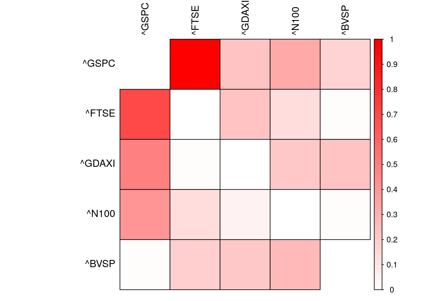
Figure 5.10: Normalized Transfer Entropy among international stock market indices.
We also calculate the marginal contribution of each market to the total Transfer Entropy in the system by calculating the sum of Transfer Entropy for each row in the Transfer Entropy matrix, which we also normalize such that all values range from 0 to 1:
TE.marginal<-base::apply(TE.matrix, 1, sum)
TE.marginal.norm<-TE.marginal/sum(TE.marginal)
print(TE.marginal.norm)
## ^GSPC ^FTSE ^GDAXI ^N100 ^BVSP
## 0.346 0.215 0.187 0.117 0.135We observe that the US is the most influential market in the time period studied detaining 34.632% of the total Transfer Entropy followed by the UK and Germany with 21.472% and 18.653%, respectively. Japan and Brazil are the least influential markets with normalized Transfer Entropies of 11.744% and 13.498%, respectively.
An experiment left to the reader is to build a daily trading strategy that exploits information flow among international markets. The proposed thesis is that one could build a profitable strategy by placing bets on futures of market indices that receive significant information flow from markets that observed unexpected returns/movements.
For an extended analysis with a broader set of indices see (Junior, Mullokandov, and Kenett 2015). The authors develop networks of international stock market indices using an information theoretical framework. They use 83 stock market indices of a diversity of countries, as well as their single day lagged values, to probe the correlation and the flow of information from one stock index to another taking into account different operating hours. They find that Transfer Entropy is an effective way to quantify the flow of information between indices, and that a high degree of information flow between indices lagged by one day coincides to same day correlation between them.
5.8 Other Applications
5.8.1 Quantifying Information Flow Between Social Media and the Stock Market
Investors’ decisions are modulated not only by companies’ fundamentals but also by personal beliefs, peers influence and information generated from news and the Internet. Rational and irrational investor’s behavior and their relation with the market efficiency hypothesis (Fama 1970) have been largely debated in the economics and financial literature (Shleifer 2000). However, it was only recently that the availability of vast amounts of data from online systems paved the way for the large-scale investigation of investor’s collective behavior in financial markets.
A research paper (Souza and Aste 2016) used some of the methods studied in this Chapter to uncover that information flows from social media to stock markets revealing that tweets are causing market movements through a nonlinear complex interaction. The authors provide empirical evidence that suggests social media and stock markets have a nonlinear causal relationship. They take advantage of an extensive data set composed of social media messages related to DJIA index components. By using information-theoretic measures to cope for possible nonlinear causal effects between social media and the stock market, the work points out stunning differences in the results with respect to linear coupling. Two main conclusions are drawn: First, social media significant causality on stocks’ returns are purely nonlinear in most cases; Second, social media dominates the directional coupling with stock market, an effect not observable within linear modeling. Results also serve as empirical guidance on model adequacy in the investigation of sociotechnical and financial systems.
Fig. 5.11 shows the significant causality links found between social media and stocks’ returns considering both cases: nonlinear (Transfer Entropy) and linear G-causality (linear VAR framework). The linear analysis discovers only three stocks with significant causality: INTEL CORP., NIKE INC. and WALT DISNEY CO. The Nonlinear analysis discovers that several other stocks have significant causality. In addition to the 3 stocks identified with significant linear causality, other 8 stocks presented purely nonlinear causality.
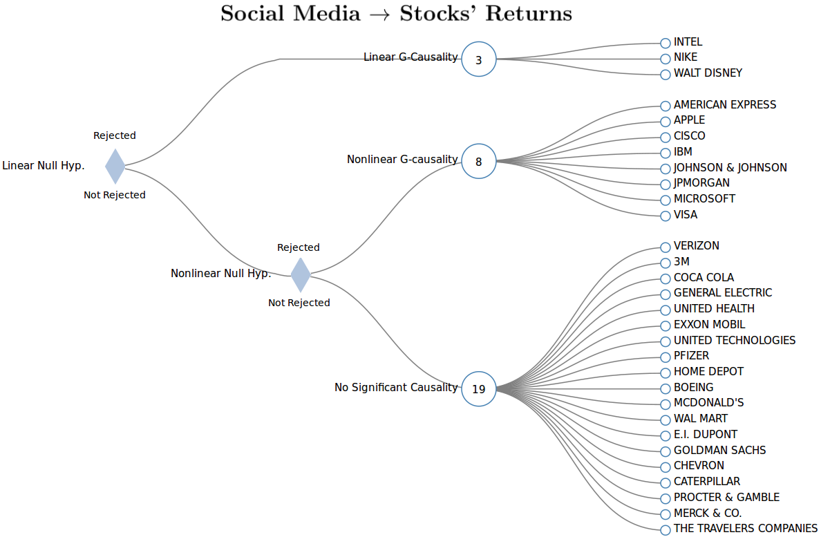
Figure 5.11: Demonstration that the causality between social media and stocks’ returns are mostly nonlinear. Linear causality test indicated that social media caused stock’s returns only for 3 stocks. Nonparametric analysis showed that almost 1/3 of the stocks rejected in the linear case have significant nonlinear causality. In the nonlinear case, Transfer Entropy was used to quantify causal inference between the systems with randomized permutations test for significance estimation. In the linear case, a standard linear G-causality test was performed with a F-test under a linear vector-autoregressive framework. A significant linear G-causality was accepted if its linear specification was not rejected by the BDS test. p-values are adjusted with the Bonferroni correction. Significance is given at p-value < 0.05.
The low level of causality obtained under linear constraints is in-line with results from similar studies in the literature, where it was found that stocks’ returns show weak causality links (Alanyali, Moat, and Preis 2013, Antweiler and Frank (2004)) and social media sentiment analytics, at least when taken alone, have small or no predictive power (Ranco 2015) and do not have significant lead-time information about stock’s movements for the majority of the stocks (Zheludev, Smith, and Aste 2014). Contrariwise, results from the nonlinear analyses unveiled a much higher level of causality indicating that linear constraints may be neglecting the relationship between social media and stock markets.
In summary, this paper (Souza and Aste 2016) is a good example on how causality can be not only complex but also misleading further highlighting the importance of choice in the methodology used to quantify it.
5.8.2 Detecting Causal Links Between Investor Sentiment and Cryptocurrency Prices
In (Keskin and Aste 2019), the authors use information-theoretic measures studied in this Chapter for non-linear causality detection applied to social media sentiment and cryptocurrency prices.
Using these techniques on sentiment and price data over a 48-month period to August 2018, for four major cryptocurrencies, namely bitcoin (BTC), ripple (XRP), litecoin (LTC) and ethereum (ETH), the authors detect significant information transfer, on hourly timescales, in directions of both sentiment to price and of price to sentiment. The work reports the scale of non-linear causality to be an order of magnitude greater than linear causality.
The information-theoretic investigation detected a significant non-linear causal relationship in BTC, LTC and XRP, over multiple timescales and in both the directions sentiment to price and price to sentiment. The effect was strongest and most consistent for BTC and LTC. Fig. 5.12 shows Transfer Entropy results between BTC sentiment and BTC prices.
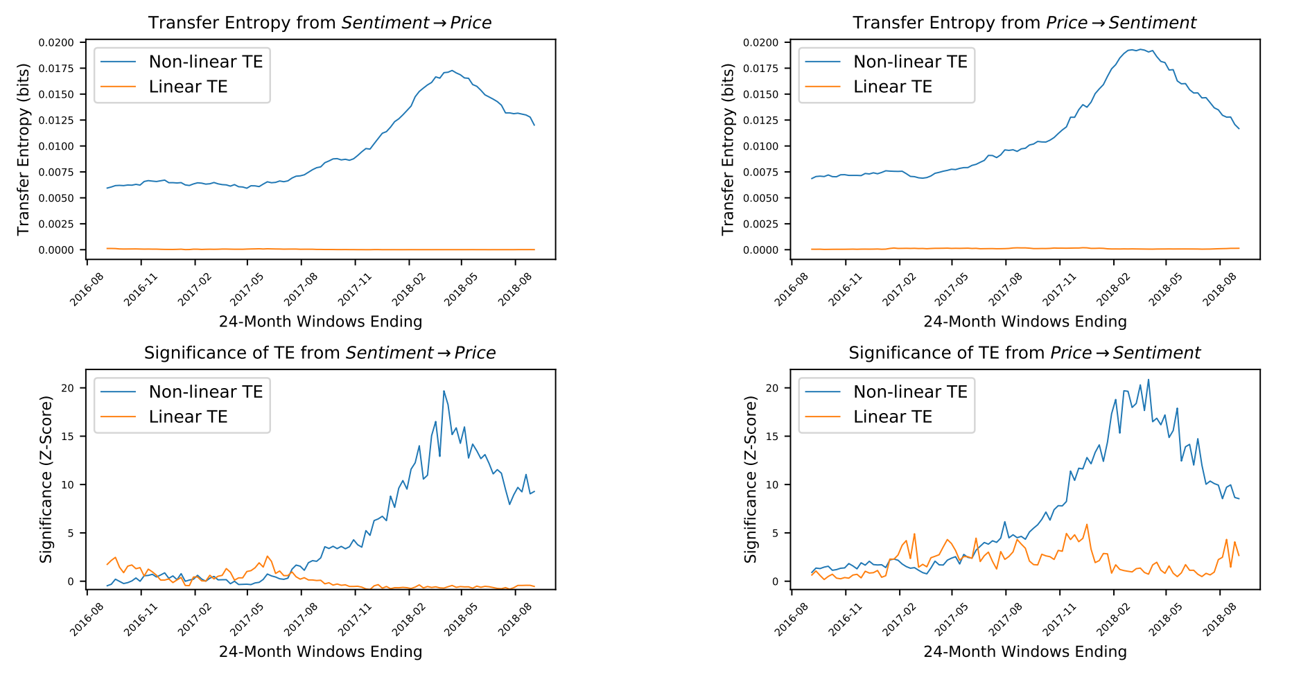
Figure 5.12: Evidence that BTC sentiment and price are causally coupled in both directions in a non-linear way. Non-linear TE is calculated by multidimensional histograms with 6 quantile bins per dimension. Z-scores, calculated over 50 shuffles, show a high level of significance, especially during 2017 and 2018, in both directions.
All analysis for this paper was performed using a Python package (PyCausality), which is available at https://github.com/ZacKeskin/PyCausality.
5.9 Conclusions
Untangling cause and effect can be devilishly difficult. However, statistical tools can help us tell correlation from causation.
In this Chapter, we introduced the notion of Granger-causality and its traditional implementation in a linear vector-autoregressive framework. We then defined information theoretical measures to quantify Transfer Entropy as a method to estimate statistical causality in nonlinear systems.
We simulated linear and nonlinear systems further showing that the traditional linear G-causality approach failed to detect simple non-linearities introduced into the system while Transfer Entropy successfully detected such relationships.
Finally, we showed how Transfer Entropy can be used to quantify relationships among global equity indexes. We also discussed further applications from the literature where Information Theoretical measures were used to quantify causal links between investor sentiment and movements in the equity and crypto markets.
We hope you enjoyed this casual causal journey and remember: Quantify causality, responsibly.
References
Alanyali, M., H. S. Moat, and T. Preis. 2013. “Quantifying the Relationship Between Financial News and the Stock Market.” Sci. Rep. 3.
Antweiler, Werner, and Murray Z. Frank. 2004. “Is All That Talk Just Noise? The Information Content of Internet Stock Message Boards.” Journal of Finance 59 (3): 1259–94.
Barnett, Lionel, Adam B. Barrett, and Anil K. Seth. 2009. “Granger Causality and Transfer Entropy Are Equivalent for Gaussian Variables.” Phys. Rev. Lett. 103 (23). American Physical Society: 238701. doi:10.1103/PhysRevLett.103.238701.
Behrendt, Simon, David Zimmermann, Thomas Dimpfl, and Franziska Peter. 2019. RTransferEntropy: Measuring Information Flow Between Time Series with Shannon and Renyi Transfer Entropy. https://CRAN.R-project.org/package=RTransferEntropy.
Fama, E. F. 1970. “Efficient Capital Markets: A Review of Theory and Empirical Work.” The Journal of Finance 25 (2). Blackwell Publishing Ltd: 383–417. doi:10.1111/j.1540-6261.1970.tb00518.x.
Granger, Clive. 1969. “Investigating Causal Relations by Econometric Models and Cross-Spectral Methods.” Econometrica 37 (3): 424–38.
Hlavackovaschindler, K., M. Palus, M. Vejmelka, and J. Bhattacharya. 2007. “Causality Detection Based on Information-Theoretic Approaches in Time Series Analysis.” Physics Reports 441 (1): 1–46. doi:10.1016/j.physrep.2006.12.004.
Junior, Leonidas, Asher Mullokandov, and Dror Kenett. 2015. “Dependency Relations Among International Stock Market Indices.” Journal of Risk and Financial Management 8 (2). Multidisciplinary Digital Publishing Institute: 227–65.
Keskin, Z, and T Aste. 2019. “Information-Theoretic Measures for Non-Linear Causality Detection: Application to Social Media Sentiment and Cryptocurrency Prices.” arXiv Preprint arXiv:1906.05740.
Michalowicz, Joseph Victor, Jonathan M. Nichols, and Frank Bucholtz. 2013. Handbook of Differential Entropy. Chapman & Hall/CRC.
Montalto, Luca AND Marinazzo, Alessandro AND Faes. 2014. “MuTE: A Matlab Toolbox to Compare Established and Novel Estimators of the Multivariate Transfer Entropy.” PLoS ONE 9 (10). Public Library of Science: e109462. doi:10.1371/journal.pone.0109462.
Ranco, D. AND Caldarelli, G. AND Aleksovski. 2015. “The Effects of Twitter Sentiment on Stock Price Returns.” PLoS ONE 10 (9). Public Library of Science: e0138441. doi:10.1371/journal.pone.0138441.
Schreiber, Thomas. 2000. “Measuring Information Transfer.” Phys. Rev. Lett. 85 (2). American Physical Society: 461–64. doi:10.1103/PhysRevLett.85.461.
Shleifer, A. 2000. Inefficient Markets: An Introduction to Behavioral Finance. Clarendon Lectures in Economics. OUP Oxford.
Souza, T. T. P., and T. Aste. 2016. “A nonlinear impact: evidences of causal effects of social media on market prices.” ArXiv E-Prints. Http://Arxiv.org/Abs/1601.04535, January. arXiv preprint. http://arxiv.org/abs/1601.04535.
Wiener, N. 1956. “The theory of prediction.” In Modern Mathematics for Engineers, edited by E. F. Beckenbach. McGraw-Hill, New York.
Zheludev, I., R. Smith, and T. Aste. 2014. “When Can Social Media Lead Financial Markets?” Scientific Reports 4 (February).