2 Introduction

Take a look at the following sections from the ggplot2 cheat sheet before reading this section.

• Coordinate systems
• Geoms: geom_bar(), geom_col(), geom_point(), and geom_count()

You’ll often want to visualize the number or amount of something across different categories. For example, you might be interested in the the number of sheep that reside in each US state, the milligrams of caffeine in different coffee drinks, or the number of distinct items exported by various countries.

We’ll call this class of visualizations “discrete-continuous” because they involve plotting a continuous variable against a discrete one. In the above examples, the states, coffee drinks, and countries are the discrete variables. The associated numbers of sheep, milligrams of caffeine, and exports are the continuous variables.

You might argue that number of sheep is not a continuous variable, as you can’t really have a fractional sheep. However, ggplot2 treats integers and doubles as continuous variables, and treats only factors, characters, and logicals as discrete.

For example, in the tibble v, y is an integer variable (the L’s create integers).

v <-
  tibble(
    x = c("a", "b"),
    y = c(1L, 2L)
  ) 

v

## # A tibble: 2 x 2
##   x         y
##   <chr> <int>
## 1 a         1
## 2 b         2

However, ggplot creates a continuous scale for y.

v %>% 
  ggplot(aes(x, y)) +
  geom_col()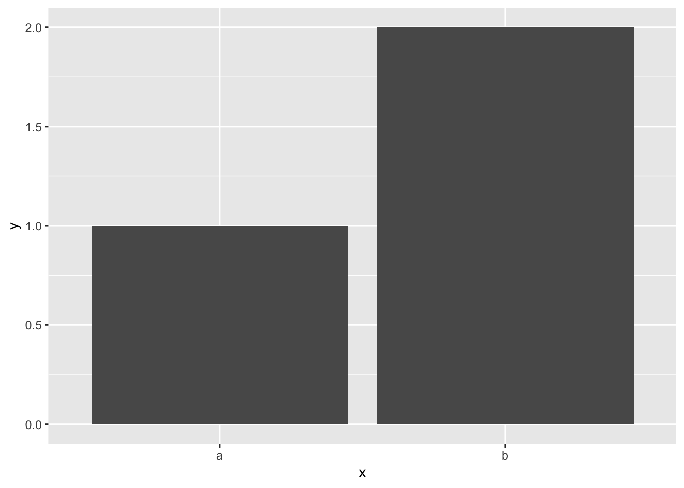

As you’ll see later, it’s useful to understand how ggplot2 treats different types of variables.

In this chapter, you’ll first learn about the mechanics of coordinate systems in ggplot2. Sometimes, you’ll want to change the default settings of a coordinate system to create a more effective visualization. You’ll need these mechanics in the “wisdom” section of the reading, where you’ll learn about common visualization strategies for discrete-continuous relationships.