1 The basics of ggplot2

The following sections from the data visualization chapter of R for Data Science (R4DS) will introduce you to the basics of plotting with ggplot2.

• Introduction
• First steps
• Aesthetic mappings
• Common problems
• Facets
• Geometric objects

Clear labelling is crucial when presenting your plots to others. The following section in R4DS introduces you to the labs() function, which allows you to edit the title, subtitle, caption, axes labels, and legend labels of your plots.

• Label

1.1 Additional information

1.1.1 Pipes and aesthetics

The above sections of R4DS create plots with code that looks like this:

ggplot(data = mpg) + 
  geom_point(mapping = aes(x = displ, y = hwy))

We instead recommend creating this plot with the following code.

mpg %>% 
  ggplot(mapping = aes(x = displ, y = hwy)) + 
  geom_point()

There are two differences. First, we’ve used %>%, which is called a pipe. The pipe takes the dataset mpg and provides it to the first argument of ggplot(), which is data. The concept of pipes is covered later in R4DS, but is useful enough to introduce here. Pipes make it easier to see which dataset is being plotted. They also allow you to easily manipulate the data before plotting. For example, you might want to apply filter() to the data before plotting.

Second, we’ve moved the aesthetics from geom_point() into ggplot(). In general, your plots will contain more than one geom. We recommend specifying the aesthetics that are shared by all of the plot’s geoms in ggplot() and specifying the aesthetics unique to a single geom in that geom call.

1.1.2 Facet syntax

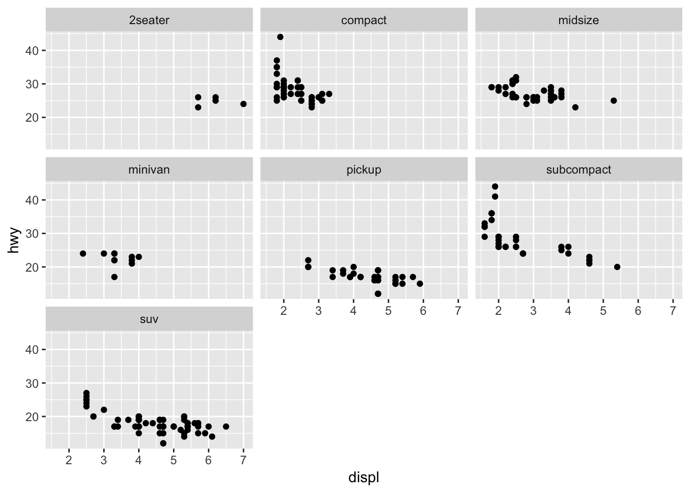
As you saw in R4DS, you can use facet_grid() and facet_wrap() to split a single plot into many.

mpg %>% 
  ggplot(mapping = aes(x = displ, y = hwy)) + 
  geom_point() + 
  facet_wrap(~ class)

The syntax for facet_grid() and facet_wrap() has been updated, however. Instead of using ~, you specify the faceting variable inside the helper function vars().

For facet_wrap(), all you have to do is replace ~ with vars().

mpg %>% 
  ggplot(mapping = aes(x = displ, y = hwy)) + 
  geom_point() + 
  facet_wrap(vars(class))

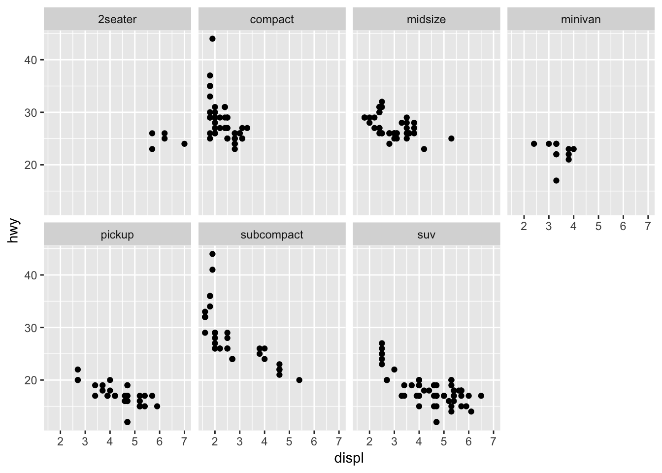
You still use the nrow and ncol arguments of facet_wrap() to control the number of rows and columns.

mpg %>% 
  ggplot(mapping = aes(x = displ, y = hwy)) + 
  geom_point() + 
  facet_wrap(vars(class), nrow = 2)

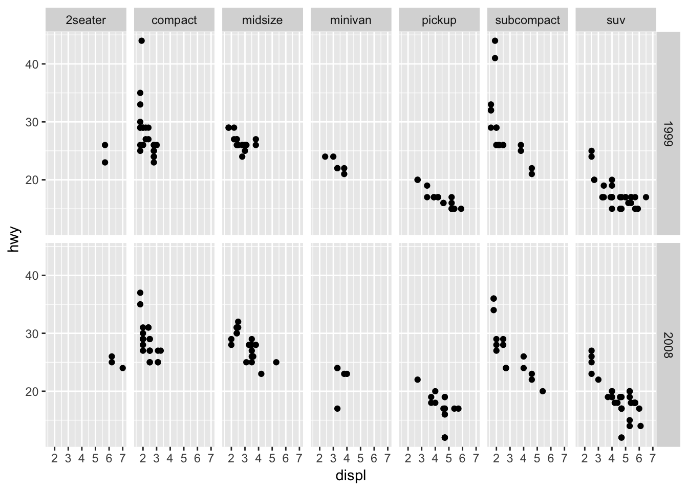
facet_grid() now has two arguments,rows and cols, that define the rows and columns of the grid.

mpg %>% 
  ggplot(mapping = aes(x = displ, y = hwy)) + 
  geom_point() + 
  facet_grid(rows = vars(year), cols = vars(class))

Again, you need to wrap the variable names in the helper function vars().