Chapter 3 Worked examples
In this chapter, short examples are given on how to apply the ASPAR_KR metadata standardisation programme. A download link to the standardised excel sheet is given at the end of each section.
3.1 Air Samples according to Kortenbosch et al. (2022).
“Following the example of Peter, we see what it takes to fill in the meta data for a limited air sample study”.
Kortenbosch et al. (2022) reports a method of cheaply taking air samples of A. fumigatus. In this technique, Delta traps are assigned to observation units and left for a certain number of days. Then the Delta traps are transferred to a flamingo agar (Zhang et al. (2021)) plate with azole, and without and the colony forming units are counted.
Peter is planning to determine the azole resistance of A. fumigatus in Arnhem vs Nijmegen. Per town, he hangs 4 air sample units, and he plans to plate them on flamingo agar and flamingo agar with itraconazole (4 mg/L).
To record these measurements using ASPAR_KR, take the following steps:
3.1.1 Set up the metadata sheet
- Go to
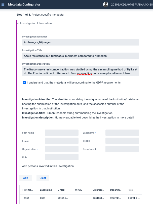
https://aspar-kr.bioinformatics.nl/template. And fill in step 1 according to Figure 3.1.- Fill in Investigation information:
- Identifier:
Arnhem_vs_Nijmegen; - Title: Azole resistance in A fumigatus in Arnhem compared to Nijmegen.
- Description: The Itraconazole resistance fraction was studied using the airsampling method of Hylke et al. The Fractions did not differ much. Four airsampling units were placed in each town.
- Identifier:
- Fill in person information (click
addwhen finished).- First name: Peter.
- Last name: Doe.
- email: peter.doe@example.com.
- Organisation: Example company.
- Role: Being a good example.
- ORCHID:
<left empty>. - Department: Example department
- Fill in Investigation information:

Figure 3.1: Filled in investigation information
Add Study information (Click:
Study information).
Since the design is simple, we can copy the information from investigation.Add the standard observational unit template.
Click:Observation unit information>Search a package>default.Fill in the experimental metadata.
Since we need to keep track of Delta traps, and their corresponding culture we use airstrip samples, and CFU count samples.- Add the AirStrip sample package:
Click:Sample Information>search a package> Scroll down and add AirStrip >Add template. - Add the CFU sample package:
Click:Sample Information>search a package> Scroll down and addCFUCountCulture>Add template. - Adjust your optional metadata requirements.
- Add the AirStrip sample package:
No assay information is needed since Peter did not plan to do genotyping or another test.
Download the excel sheet (
Generate workbook). You can download the resulting sheet here, to circumvent steps 1-5.
3.1.3 The common metadata tables
As mentioned in Section 2.1, between each class, objects are linked by identifiers. In the Arnhem_vs_Nijmegen.xlsx sheet things are no different, you’ll find the following 5 tables in this sheet:
Table 3.1: The investigation. Links to Study via investigation identifier.
Table 3.2: The study. Links to observational unit via study identifier.
Table 3.3: The observational unit. Links to Sample via observational unit identifier.
These three tables will always be present. The actual research data will is always part of the sample and assay tables.
| investigation identifier | investigation title | investigation description | firstname | lastname | email address | orcid | organization | department |
|---|---|---|---|---|---|---|---|---|
| Arnhem_vs_Nijmegen | Azole resistance in A fumigatus in Arnhem compared to Nijmegen. | The Itraconazole resistance fraction was studied using the airsampling method of Hylke et al. The Fractions did not differ much. Four airsampling units were placed in each town. | Peter | Doe | p.p@ex.com | org | s |
| study identifier | study description | study title | investigation identifier |
|---|---|---|---|
| Arnhem-vs-nijmegen | 4 samples in each town were made using hylkes method | Azole resistance in A fumigatus in Arnhem compared to Nijmegen. | Arnhem_vs_Nijmegen |
| observation unit identifier | observation unit name | observation unit description | study identifier |
|---|---|---|---|
| arnhem | Arnhem | Measurements in Arnhem | Arnhem-vs-nijmegen |
| nijmegen | Nijmegen | Measurements in Nijmegen | Arnhem-vs-nijmegen |
3.1.4 Experimental data tables
3.1.4.1 Air samples
To fill in these tables Peter hangs the Air sample strips up for 4 weeks: between the 5th of November and the 26th of November. He records the minimal information for the air sample strips:
start end end date.
Collection location.
- Lat
- Long
For taxonomy ID he picks 32644: unidentified, since Peter does not know which species he will collect on his Delta Trap. For the culture made using the Delta Trap, he selects for A. fumgiatus, so 746128
He also collects the recommended and optional data:
- Altitude
- Environmental context:
- Broad scale.
Overall environment where the sample is found? What has the biggest influence on the environment of the sample? - Local scale.
Things in the vicinity of the sample that may influence the outcome of the experiment. - Environmental medium.
Things that directly surrounded your sample prior to sampling.
- Broad scale.
In Arnhem & Nijmegen he hangs some samples in trees of the the park, others at the train station at traffic poles. Since he wants to record these terms as part of the environmental contex, he looks up the terms on ontobee/envo (Figure 3.2). He finds that:
- The Broad scale environmental context is “City”
- The local environmental context is “Road” or “Park”.
- The medium for samples in a park is “tree” and for the train station: “pole”.
.](graphs/ontobee-road.png)
Figure 3.2: Lookup of a machine readable term on Ontobee.
Using this information, he fills in the Delta Trap excel sheet.
3.1.4.2 Culture Samples
After filling in the air sample sheet, he fills in the information for the two layer culture:
As a selection medium, he adds itraconazole to a concentration of 4 g/L (\(x\) molar)1, which has CHEMBL1835949 as the standard identifier.
3.1.5 Convert the sheet to ttl format
- Go to
https://aspar-kr.bioinformatics.nl/validate. - Upload the finalised sheet.
- Click “DOWNLOAD RDF”.
3.1.6 Analysis of the FAIR data with R
To analyse the data we can use the rdflib package in R together with the tidyverse.
base::dir.create("hylke_air_method_example")
destfile="./hylke_air_method_example/data.ttl"
 fileURL <-
 "https://git.wur.nl/aspar_kr/aspar/-/raw/main/example_files/Arnhem_vs_Nijmegen.ttl?ref_type=heads"
 if (!base::file.exists(destfile)) {
    utils::download.file(fileURL ,destfile,method="w")
 }

rdf <- rdflib::rdf_parse("hylke_air_method_example/data.ttl",
                         format = "turtle")
rdf
## Total of 416 triples, stored in hashes
## -------------------------------
## <http://fairbydesign.nl/ontology/inv_arnhemVsNijmegenComparison/stu_arnhemVsNijmegen/obs_nijmegenAirSamples/sam_CultureNijmegenStation2> <http://fairbydesign.nl/ontology/biosafety_level> "2"^^<http://www.w3.org/2001/XMLSchema#integer> .
## <http://fairbydesign.nl/ontology/inv_arnhemVsNijmegenComparison/stu_arnhemVsNijmegen/obs_nijmegenAirSamples/sam_CultureNijmegenStation2> <http://schema.org/description> "A two layer culture made from the delta trap taken from the station square in Nijmegen" .
## <http://fairbydesign.nl/ontology/inv_arnhemVsNijmegenComparison/stu_arnhemVsNijmegen> <http://schema.org/identifier> "arnhemVsNijmegen" .
## <http://fairbydesign.nl/ontology/selection_medium> <http://www.w3.org/1999/02/22-rdf-syntax-ns#type> <http://www.w3.org/1999/02/22-rdf-syntax-ns#Property> .
## <http://fairbydesign.nl/ontology/inv_arnhemVsNijmegenComparison/stu_arnhemVsNijmegen/obs_nijmegenAirSamples/sam_CultureNijmegenPark1> <http://fairbydesign.nl/ontology/antibiotics> "CHEMBL1835949" .
## <http://fairbydesign.nl/ontology/inv_arnhemVsNijmegenComparison/stu_arnhemVsNijmegen/obs_arnhemAirSamples/sam_CultureArnhemStation2> <http://www.w3.org/1999/02/22-rdf-syntax-ns#type> <http://jermontology.org/ontology/JERMOntology#Sample> .
## <http://fairbydesign.nl/ontology/biosafety_level> <http://schema.org/valueRequired> "true"^^<http://www.w3.org/2001/XMLSchema#boolean> .
## <http://fairbydesign.nl/ontology/inv_arnhemVsNijmegenComparison/stu_arnhemVsNijmegen/obs_nijmegenAirSamples/sam_CultureNijmegenStation2> <http://www.w3.org/1999/02/22-rdf-syntax-ns#type> <http://jermontology.org/ontology/JERMOntology#Sample> .
## <http://fairbydesign.nl/ontology/inv_arnhemVsNijmegenComparison/stu_arnhemVsNijmegen/obs_nijmegenAirSamples/sam_CultureNijmegenStation2> <http://fairbydesign.nl/ontology/medium_type> "flamingo medium" .
## <http://fairbydesign.nl/ontology/inv_arnhemVsNijmegenComparison/stu_arnhemVsNijmegen/obs_arnhemAirSamples/sam_arnhem2> <http://fairbydesign.nl/ontology/packageName> "DeltaTrap" .
##
## ... with 406 more triplesAfter reading the RDF object we can perform simple SPARQL queries to get tibble data.
sparql_query <-
  ' # Select the first 5 of everything...
  SELECT * WHERE {?s ?p ?o} LIMIT 5
  '
result <- rdflib::rdf_query(rdf, sparql_query)
result
## # A tibble: 5 × 3
## s p o
## <chr> <chr> <chr>
## 1 http://fairbydesign.nl/ontology/inv_arnhemVsNijmegenComparison/st… http… 2
## 2 http://fairbydesign.nl/ontology/inv_arnhemVsNijmegenComparison/st… http… A tw…
## 3 http://fairbydesign.nl/ontology/inv_arnhemVsNijmegenComparison/st… http… arnh…
## 4 http://fairbydesign.nl/ontology/selection_medium http… http…
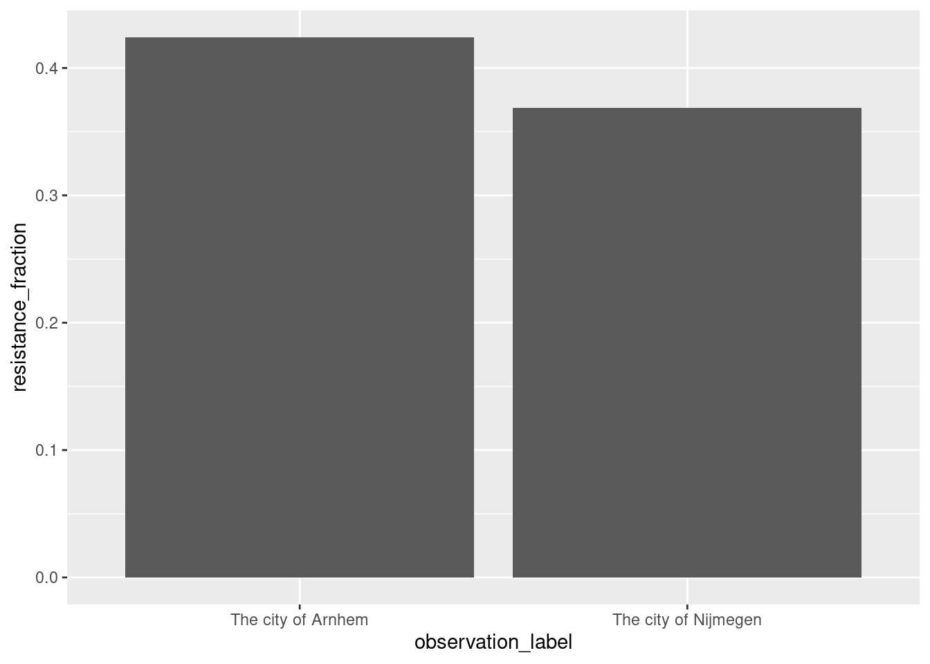
## 5 http://fairbydesign.nl/ontology/inv_arnhemVsNijmegenComparison/st… http… CHEM…Now, to plot an overview of Peter’s experiment we can use:
sparql_query <-

  ' # Select the first 5 of everything...
  prefix ppeo:     <http://purl.org/ppeo/PPEO.owl#>
  prefix jerm:     <http://jermontology.org/ontology/JERMOntology#>
  prefix fair:     <http://fairbydesign.nl/ontology/>
  prefix rdfs:     <http://www.w3.org/2000/01/rdf-schema#>
  prefix schema:   <http://schema.org/>
  SELECT ?observation_label ?sample_label (COUNT(?sample_label) as ?n) ?total_cfu ?selection_cfu WHERE {
    # Get the samples of interest
    ?observation_unit a ppeo:observation_unit .
    ?observation_unit jerm:hasPart ?parts .
    ?parts a jerm:Sample .
    ?parts fair:packageName "TwoLayerCulture" .
    ?observation_unit schema:name ?observation_label .
    ?parts schema:name ?sample_label .

    # Experimental data
    ?parts fair:total_cfu ?total_cfu .
    ?parts fair:selection_cfu ?selection_cfu .
  } GROUP BY ?observation_unit
  '
result <- rdflib::rdf_query(rdf, sparql_query)
result
## # A tibble: 2 × 5
## observation_label sample_label n total_cfu selection_cfu
## <chr> <chr> <dbl> <dbl> <dbl>
## 1 The city of Arnhem Arnhem Centraal culture 4 66 28
## 2 The city of Nijmegen Nijmegen stationsplein cul… 4 57 21The result table, we can modify and plot using the tidyverse.
result |>
  dplyr::mutate(resistance_fraction = selection_cfu / total_cfu) |>
  ggplot2::ggplot(ggplot2::aes(x = observation_label, y = resistance_fraction)) +
  ggplot2::geom_bar(stat="identity")
References
Molecular weight of itraconazole is 705.6 g/mol, he added 4 g to 1 liter of flamingo medium. Therefore
((1 * mole) / (705.6 * gram)) * (4 * gram) = approx. 5.6689342 mmol.↩︎