B Tidy data and data exploration
In this chapter, we begin with the principles of tidy data, which outline how data should be organized to facilitate data exploration and analysis. With these principles in mind, we learn how to create a data frame in R and how to import rectangular tables with the help of the readr package, specifically the read_csv() function. In the final part of the chapter, we learn basic “verbs” from the the dplyr package that help us wrangle data and in so doing learn how data exploration works in R.
Prerequisite
In this chapter, we will make use of core packages from the tidyverse (i.e., readr and dplyr), so go ahead and load the packages.
library(tidyverse)

# Alternatively load each one separately
library(dplyr)
library(readr)
Principles of tidy data
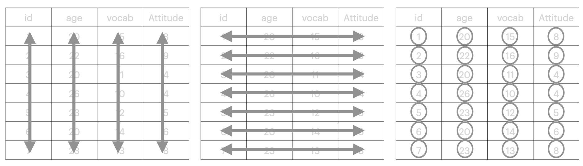
Data come in various forms and sizes. Most data that we input into spreadsheet programs such as Excel and Google Sheets are rectangular tables. As the name implies, rectangular tables are shaped like a rectangle, consisting of rows and columns. The two tables below are examples of rectangular tables:
table1## # A tibble: 7 × 4
## id age vocab attitude
## <int> <dbl> <dbl> <dbl>
## 1 1 20 15 8
## 2 2 22 16 9
## 3 3 20 11 4
## 4 4 26 10 4
## 5 5 23 12 5
## 6 6 20 14 6
## 7 7 23 13 8table2## # A tibble: 14 × 4
## id age test_type scores
## <int> <dbl> <chr> <dbl>
## 1 1 20 vocab 15
## 2 1 20 attitude 8
## 3 2 22 vocab 16
## 4 2 22 attitude 9
## 5 3 20 vocab 11
## 6 3 20 attitude 4
## 7 4 26 vocab 10
## 8 4 26 attitude 4
## 9 5 23 vocab 12
## 10 5 23 attitude 5
## 11 6 20 vocab 14
## 12 6 20 attitude 6
## 13 7 23 vocab 13
## 14 7 23 attitude 8We can see that the two tables represent the same data, notwithstanding the number of rows and columns. That is, each table contains test scores of some participants. Looking closely at the two tables, we may see that each participant provides two sets of scores: vocabulary and attitude.
But these two tables are not equally tidy! Table1 presents data in a more easy-to-use way and it is a tidy dataset. In contrast, Table2 is less tidy and will require a bit of work before it is ready for data analysis. In Table1, we can see key principles of tidy data, which are:
- Each variable has its own column (e.g.,
id,age,vocab, andattitude); - Each observation is in its own row (e.g.,
1,20,15and8); and - Each value must have its own cell (e.g., a vocabulary score of 15, not 15/30).
These principles can be graphically represented as:
Exercise:
Look at the following spreadsheets. Are they tidy? If not, what can we do to fix them?
- Spreadsheet 1
- Spreadsheet 2
- Spreadsheet 3
Data frames and tibbles
In R, rectangular data (like spreadsheets) are represented by data frames. We can create a data frame with the function data.frame() from Base R. In this function, we must specify one argument, that is a set of column names and their values.
dat <- data.frame(Class  = c("A", "A", "A", "B", "B", "B"),
                  Gender = c("M", "F", "M", "F", "F", "M"),
                  Test   = c(15, 20, 21, 16, 17, 18)
                  )
If data frames look to you like a combination of vectors, you are not crazy! Technically speaking, data frames are a named list of vectors. One important constraint of data frames is that the length of each vector in a data frame must be the same. In dat above, all vectors have a length of 6.
We can inspect the structure of a data frame with the function str(), which compactly displays the internal structure of a data frame (or any other objects).
str(dat)## 'data.frame': 6 obs. of 3 variables:
## $ Class : Factor w/ 2 levels "A","B": 1 1 1 2 2 2
## $ Gender: Factor w/ 2 levels "F","M": 2 1 2 1 1 2
## $ Test : num 15 20 21 16 17 18We can see, on each line, a column name, type, and first few elements of the “vector”. We can also see how many rows and columns a data frame has with: nrow() and ncol(). The function length() will give the number of columns.
Another useful function, which provides a descriptive summary, is:
summary(dat)## Class Gender Test
## A:3 F:3 Min. :15.00
## B:3 M:3 1st Qu.:16.25
## Median :17.50
## Mean :17.83
## 3rd Qu.:19.50
## Max. :21.00And, finally, we can peak inside data frames with two functions head() and tail():
head(dat, n = 3)
tail(dat, n = 3)
Tidyverse provides an extremely useful function tibble() to create tibbles (aka data frames). Tibbles are more or less data frames. There are certainly some big differences between the two, but we are not going to focus on those here. Interested readers should check out Hadley Wickham’s Advanced R chapter on tibbles.
tib <-tibble(Class  = c("A", "A", "A", "B", "B", "B"),
             Gender = c("M", "F", "M", "F", "F", "M"),
             Test   = c(15, 20, 21, 16, 17, 18)
             )
Reading spreadsheet files into R
We can input our data into R with data.frame() or tibble(). But in most cases, our data may be hundreds of rows long, if not more. It would be unwise to manually enter data into R since doing so may be error-prone. In other instances, we may work with a team of data scientists and our team may prefer to use spreadsheet programs like Excel or Google Sheets to save data.
We can easily read these files into R with the help of readr package. There are several functions to import various types of files (e.g., read_delim() and read_csv()). We can also load the readxl package (which is part of the Tidyverse but is not loaded explicitly) to make use of its functions read_xls() and read_xlsx(). In this chapter, we are going to focus solely on read_csv(), which is designed to read a comma-separated value (csv) file.
Before we learn how to import files into R, go ahead and download the SPI Data file from the following website. Once you download the file, move it to your project’s folder. If you are not sure where you are, use getwd() to obtain your current working directory:
getwd()To import a csv file with read_csv(), the most important argument we need is a path to the file, specified in file = "<name>"
# Provide a file path
spi <- read_csv(file = "spi_modified.csv")

# Provide a relative path to the folder "Data"
spi <- read_csv(file = "./Data/spi_modified.csv")| Use forward slashes (/) for path, regardless of your computer’s OS (Mac or Windows) |
Another important argument is col_names which readr will use to specify column names. We can provide a character vector to col_names which will be used as column names
# Default behavior
spi <- read_csv(file = "spi_modified.csv",
                col_names = TRUE)

# What does this code do?
spi <- read_csv(file = "spi_modified.csv",
                col_names = FALSE)


# DO NOT RUN: Vector length not equal to columns
spi <- read_csv(file = "spi_modified.csv",
                col_names = c("a", "b", "c")
                )
Another option that we can tweak as we import files into R is na, which tells readr what value(s) represent(s) missing values in the file:
# Default behavior
spi <- read_csv(file = "spi_modified.csv",
                col_names = TRUE,
                na = c("", "NA")
                )

# Omit na if there's no missing value or
spi <- read_csv(file = "spi_modified.csv",
                col_names = TRUE,
                na = character()
                )

# If your na is coded as something else (e.g., 999)
# Pass that number as character string
spi <- read_csv(file = "spi_modified.csv",
                col_names = TRUE,
                na   = c("NA", "999")
                )
Thus far, we have ignored the message that read_csv() prints out to the console. What read_csv() (and other functions in the readr package) essentially tells us is that it tries to figure out what type each column of the file is. We can provide specific column type to read_csv() with col_types:
# DO NOT RUN: Example
spi <- read_csv(file = "spi_modified.csv",
                col_names = TRUE,
                na   = c("NA", "999"),
                col_types = cols(
                  country = col_character(),
                  date = col_date()
                  )
                )
if we want to be explicit about column types in only one or two columns, provide those types in col_types and leave the rest to read_csv() to work out.
Extra bits: Importing files from the Internet
In a few instances, we may wish to download csv files (or any other types) from the internet. For instance, as part of our analysis, we may need to import a few files hosted on a site (such as this one). This can be done quite easily:
twin <- read_csv(file = "https://courses.washington.edu/b517/Datasets/TWINS.csv",
                col_names = TRUE
                )
Extra bits: Importing files with unicode characters
We can also import spreadsheets with non-English characters. readr yields character strings encoded in UTF-8. The easiest way to read in non-English files is to save them as a csv file with UTF-8. Then, we can simply call read_csv():
# DO NOT RUN: Example
covid_thailand <- read_csv(file = "covid_Feb2022.csv",
                           na = c("")
                           )

# DO NOT RUN: Fix the problem when file imported
problems(covid_thailand)
Data wrangling
Now that we have our files in R, let’s focus on key “verbs” in the dplyr package. These verbs are designed to help us explore data to gain deeper insights. For didactic purposes, we are going to focus on data frames that are part of Tidyverse. Once you get a hang of these verbs, you can easily apply them to your own data frames.
data(diamonds)# Explore the diamond dataset
str(diamonds)
summary(diamonds)While str() and summary() give us some useful information about the diamond dataset, they cannot answer all of our needs. In a few cases, we may want to, for instance:
- subset a large data frame based on some information in columns x or y;
- select only a few columns from the whole data frame; or
- calculate summary statistics by groups.
To address these data manipulation challenges, we will need to learn several verbs in dplyr. Each verb performs a specific function:
| Verbs | Functions | Examples |
|---|---|---|
filter() |
select rows by their values | filter(diamonds, x > 3.85) |
select() |
select columns | select(diamonds, carat, cut) |
relocate() |
changes column positions | relocate(diamonds, depth) |
arrange() |
sorts rows by their values | arrange(diamonds, x) |
mutate() |
creates new columns | mutate(diamonds, dim = x*y*z) |
summarize() |
combines values to form a new one | summarize(diamonds, M = mean(x)) |
These verbs are consistent; each function has the same “format”. That is, the first argument of each verb takes a name of the data frame (e.g., diamond) and the second argument accepts a list of column names, without quote.
We will go through each “verb” one by one. For each verb, we will also look at some helper functions. Later, we will string all these verbs together with %>% (pipe), and we will get a long line of codes that can complete some useful data manipulation challenges.
1. select()
select() is useful when you want to subset columns. There are four ways to use select():
- pick columns by their names;
- pick columns by their numbers;
- pick columns by functions; and
- pick columns by types
Firstly, you can pick columns by their names with select(). You specify which columns you would like to select without quotes. By default, columns that are not selected will be dropped:
diamonds
select(diamonds, x, y, z)
select(diamonds, c(x, y, z) )
Like every other verb in the dplyr package, select() always returns a tibble. If you want to create a new tibble from select(), you can assign the “result” of select() to a new variable:
diamonds_small <- select(diamonds, c(x, y, z)
                         )
You can specify a range of columns with a colon (:) inside select(). As the example below shows, x:z is equivalent to x, y, z:
# The two commands are the same
select(diamonds, x, y, z)
select(diamonds, x:z)
Exercise:
Run the following codes. Which columns are selected?
select(diamonds, -depth)
select(diamonds, -c(depth, table))
select(diamonds, !x)
select(diamonds, !c(x, z))
Secondly, you can pick columns by their numbers with select(), though this approach is generally not recommended.
select(diamonds, 1, 3, 5)
select(diamonds, c(1, 3, 5) )
select(diamonds, 1:3)
Thirdly, you can use helper functions to select columns:
| Functions | What it does |
|---|---|
starts_with("car") |
select columns that starts with “car” |
ends_with("ty") |
select columns that end with “ty” |
matches("\\d.+") |
select columns with regular expressions |
contains("car") |
select columns with “car” in the name |
everything() |
select all columns |
Complete the following exercises to help you better understand the helper functions.
Exercise:
Write codes to perform the following actions. You may combine helper functions with - and : to select columns:
Select
carat,cut,color, andclarityfromdiamonds;Select
carat, andcut;Select
depth,table,price,x,y, andz; andSelect
tableandprice
And finally, select() can be used to pick columns by types. Notice the use of where() along with is.*() functions
select(diamonds, where(is.numeric) )
select(diamonds, where(is.factor) )

# What happens here?
select(diamonds, where(is.character) )
We can combine these four options with Boolean operators (&, | or !) to select columns.
select(diamonds, starts_with("c") & where(is.factor) )

select(diamonds, starts_with("c") & !where(is.factor) )
2. relocate()
Sometimes, we may need to change column positions relocate() is designed to help us do accomplish this easily by moving one or multiple columns at once. The same four approaches to selecting columns we looked at above apply:
relocate(diamonds, clarity)
relocate(diamonds, clarity, depth)
relocate(diamonds, 3:5)
relocate(diamonds, ends_with("e") )
relocate(diamonds, where(is.numeric) )
relocate(diamonds, starts_with("c") & where(is.factor)
         )
Columns that are explicitly named inside relocate() are moved to the front of the data frame. We can tell relocate() where we want the columns to go with .before = and .after = arguments:
relocate(diamonds, x, .before = cut)
relocate(diamonds, x, .after = cut)    #but notice:
relocate(diamonds, x, .before = cut, .after = carat)
We can combine the two verbs in order to subset diamonds and change column positions. At each stage, we assign the outcome to the data frame small_dia.This two-step process works because each verb takes and returns a data frame.
small_dia <- select(diamonds, starts_with("c") &
                      where(is.factor), x:z
                    )

small_dia <- relocate(small_dia, x:z, .before = color)
Before we move on to the next verb, it’s worth pointing out that select() subsets our data, narrowing them down to only those columns we specify, while relocate() returns a tibble with the same number of columns (and rows) as the original one. Run the code below to see what happens:
select(diamonds, where(is.numeric) )
relocate(diamonds, where(is.numeric) )
3. filter()
While select() helps us pick columns, filter() lets us pick observations (i.e., rows). With filter(), we subset and retain rows that meet our condition(s). We are going to work with a new data frame known as mpg. The dataset is adapted from data made available by the Environmental Protection Agency (EPA). In mpg, each row represents a car model released between 1999 and 2008.
data(mpg)
help(mpg)
We can specify a condition we wish to keep. For instance, we may only want to analyze data from 6-cylinder cars. Because this information is under cyl (i.e., number of cylinders), we provide the condition inside filter that meets our criterion (i.e., cyl > 6):
filter(mpg, cyl > 6)
filter(mpg, cyl < 6)
filter() works with comparison operations we saw previously:
filter(mpg, manufacturer  == "nissan")
filter(mpg, manufacturer  == "nissan" | manufacturer  == "subaru")

filter(mpg, hwy >= 22)

filter(mpg, hwy > 20 & hwy < 30)

# Or use between()
filter(mpg, between(hwy, 20, 30))
In the second line of code above, we use | to select either nissan or subaru. A useful shorthand for this is %in%:
filter(mpg, manufacturer  %in% c("nissan", "subaru") )

filter(mpg, !manufacturer %in% c("nissan", "subaru") )
And of course, you can combine more than one condition in filter():
filter(mpg, year == 2008,  cyl == 6)   #same as
filter(mpg, year == 2008 & cyl == 6)
filter(mpg, year == 1999 | cyl != 6)
Exercise:
Find cars that…
are manufactured by Toyota or Honda;
are made by Toyota or Honda and have 4 cylinders;
are SUV and can get 15 miles or more per gallon in city;
are four-wheel drive SUV; and
run 17 miles an hour in city and 20 miles an hour on highway.
One thing we haven’t discussed more thoroughly is NA:
#NA is unknown
NA > 5
NA == NA
nums <- c(15, 20, 23, 24, NA, 26, NA, 31)

# NA is contagious
mean(nums)
sd(nums)
max(nums)
To check if elements inside a vector are NA, use is.na():
nums <- c(15, 20, 23, 24, NA, 26, NA, 31)
is.na(nums)
In several functions, you can remove NA with na.rm = TRUE
mean(nums, na.rm = TRUE)
sd(nums, na.rm = TRUE)
filter() only includes rows that are TRUE of your condition(s). If you want rows with NA, you’ll need to use is.na():
filter(covid_thailand, nationality == "Thailand")
filter(covid_thailand, nationality == "Thailand" | is.na(nationality) )

# what's going on here?
filter(covid_thailand, nationality == "Thailand" & is.na(nationality) )
At this point, we can begin to combine the two verbs select() and filter() together to retrieve specific pieces of information from a data frame. We can choose to complete each step and assign an end product to a new data frame, just as we did previously with select() and relocate(). Alternatively, we can nest one verb inside another. For instance, we may wish to know which car models in 2008 could drive more than 30 miles per gallon:
select( filter(mpg, year == 2008 & hwy >= 30),
        c(manufacturer, model)
        )
What does this code do? We begin by telling R to filer the data frame mpg by picking observations that come from the year 2008 and that have highway miles per gallon equal to or greater than 30. Then, a resulting data frame is fed through select() which picks the two columns manufacturer and model and drop the rest of the columns.
Notice that we nest filter() inside the select() operation, and this means that the filter() operation is evaluated first. Contrast the above code with the following:
filter( select(c(manufacturer, model) ),
        mpg, year == 2008 & hwy >= 30
        )
Why doesn’t the second code work? Go through each verb slowly to figure out what went wrong.
4. mutate()
So far, we have learned how to select columns and rows that meet our condition(s). But in other instances, we may want to add new columns to existing tibbles. For instance, we may want to have a column that records the source of our data frame. To achieve this, we are going to use mutate() and provide an argument "<names>" = ... inside it:
#create a column that repeats "EPA"
mutate(mpg, source = "EPA")

#or add this column back to the tibble
mpg_new <- mutate(mpg, source = "EPA")
We can see that EPA is repeated 234 times. But why? If you recall, arithmetic operation is vectorized in R:
(num1 <- 1:10)
##  [1]  1  2  3  4  5  6  7  8  9 10

num1 + c(2,4)
##  [1]  3  6  5  8  7 10  9 12 11 14

num1 + 15
##  [1] 16 17 18 19 20 21 22 23 24 25
R expands a shorter vector to match the length of a longer one. This means that our source = "EPA" is expanded to match the length of mpg. Also, if you recall, R does arithmetic operations on two vectors element-wise:
c(5, 6, 7, 8, 9) + c(10, 11, 12, 13, 14)
## [1] 15 17 19 21 23
We can apply this principle to our data frame. For instance, we can create a new column that represents the difference between the number of miles a car can run in the city vs. on the highway.
mutate(mpg, dif = hwy - cty)

#or add to an existing tibble
mpg_small <- mutate(mpg, dif = hwy - cty)
You can reference a newly created variable right inside mutate():
mutate(mpg, dif = hwy - cty,
       dif_percent = dif / 100
       )
Exercise:
Create new variables that…
subtract
hwyfrom the maximum value ofhwy;subtract
hwyfrom the average ofhwy;convert the number of miles in
ctyandhwyto kilometers
Arithmetic operations can serve us well with numeric vectors. But in many other instances, we may want to create a new column based on some condition in an existing column. For instance, we may want to divide cars into those that are “big” cars (with 6 or more cylinders) or small cars (with 6 or fewer cylinders). A useful function to help us accomplish this is if_else():
gen    <- rep(c("M", "F"), times = 5)
scores <- 11:20


#dplyr::if_else(condition, true, false)
if_else(gen == "F", "female", "male")
if_else(scores > mean(scores), "above", "below")
Exercise:
Create new variables from mpg that…
re-code
yearfrom 1999 to “90s” and from 2008 to “00s”;classify
ctyinto “above” and “below” based onmean(cty, na.rm = T);change only “suv” in
classinto “big car”
Complete the following steps with the mpg data frame:
Create a subset of
mpgthat consists ofmanufacturer,model,year,cyl,cty, andclass;Move the
yearcolumn to the front;Add a new column that converts mpg in
ctyto kpg; andDrop the original
ctycolumn.
This exercise should hopefully highlight some of the things we do to wrangle and explore data. Using what we have learned so far, we may accomplish these tasks in four steps:
mpg_small <- select(mpg, starts_with("m"),
                         year,
                         starts_with("c")
                    )

mpg_small <- relocate(mpg_small, year)

mpg_small <- mutate(mpg_small, cty_k = cty * 1.61)

mpg_small <- select(mpg_small, !cty)
Note that we modify mpg_small several times. What could possibly go wrong with that? Long story short, we may accidentally misspell a data frame name (e.g., mpg_smal instead of mpg_small). If this happens, R will likely throw an error at us when we try to call mpg_small. To prevent this from happening, we may choose to pursue another option, creating a new variable at each intermediate step:
mpg_small <- select(mpg, starts_with("m"),
                         year,
                         starts_with("c")
                    )

mpg_small2 <- relocate(mpg_small, year)

mpg_small3 <- mutate(mpg_small2, cty_k = cty * 1.61)

mpg_small4 <- select(mpg_small3, !cty)
But this approach isn’t ideal either. With new data frame at each step, the Environment becomes cluttered. There are too many data frames that we are not interested in keeping. We’d like to combine these incremental steps into one big chunk of codes that shows the transformations, rather than what is getting transformed. Moreover, we want to be able to show the pipeline of our code.
We are going to do that with %>% (meaning “and then”) from the package magrittr which tidyverse has access to. From now on, we are going to make use of %>% all the time, so it’s worth remembering a keyboard shortcut for it. It is command+shift+m on Mac and clt+shift+m on Windows computers.
library(magrittr)We start with a data frame and pipe it into a series of commands. For instance, if we want to select manufacturer, model, year, cyl, cty, and class from the data frame mpg, we can write:
mpg %>%
  select(starts_with("m"), year, starts_with("c"))

# Equivalent to
select(mpg, starts_with("m"), year, starts_with("c"))
We can then pipe the output of the first step into the next with another %>% (and then another pipe and on and on)!
mpg %>%
  select(starts_with("m"), year, starts_with("c")
         ) %>%
  relocate(year) %>%
  mutate(cty_k = cty * 1.61) %>%
  select(!cty)
And if we want to save this into a new data frame, it is extremely easy:
mpg_new <- mpg %>%
  select(starts_with("m"), year, starts_with("c")
         ) %>%
  relocate(year) %>%
  mutate(cty_k = cty * 1.61) %>%
  select(!cty)
Exercise:
- Describe what the following code does.
mpg_small <- mpg %>%
  select(starts_with("m"),
         where(is.numeric)
         ) %>%
mutate(hwy_dif = max(hwy) - hwy)- What is wrong with this line of codes?
mpg_small <- mpg %>%
  select(starts_with("m")
         ) %>%
  select(!cty)
With %>% in our toolkit, let’s talk about group_by(). Previously we created a new column with mutate() that converted miles into kilometers row by row. While this is certainly useful, there are instances where such an operation will not be enough. For example, we may want to know if a car consumes less gas on average with respect to other cars in the same category. More specifically, we may want to find out if a Honda civic is above average or below average when compared with other cars in the subcompact class. To find out, we will need an average of each class:
mpg_new <- mpg %>%
  group_by(class) %>%
  mutate(difference = ctw - mean(cty, na.rm = T)
         )
group_by() takes a data frame (mpg in this example) and folds it into groups (by class here). Then, for each class, it creates a new column that finds the difference between each particular row and its average. If this still sounds confusing, run the codes below. Don’t worry about what summarize() does; we will talk about it later.
mpg %>%
  group_by(class) %>%
  summarize(M = mean(cty, na.rm = T)
            )

mpg %>%
  summarize(M = mean(cty, na.rm = T)
            )
5. summarize()
While mutate() creates new columns by adding “things” to each row of a tibble, summarize() collapses a column into a single row:
mpg %>%
  summarize(ave_cty = mean(cty),
            ave_hwy = mean(hwy)
            )
summarize() operates on the whole column. If we’d like to get a summary by groups (or conditions or units), we can pair summarize() with group_by(). We can group by multiple variables to roll up our data.
mpg %>%
  group_by(manufacturer) %>%
  summarize(ave_cty = mean(cty),
            ave_hwy = mean(hwy)
            )
Exercise:
Find the average and standard deviation of
ctybymanufacturerandclass;Find the maximum value of
hwybyyear,manufacturer, andcyl(cylinders);Count the number of cars by manufacturer and class
To count how many “items” there are, we can use n(). In fact, n() is just one of the many useful count functions that work well with summarize():
mpg %>%
  group_by(manufacturer, class) %>%
  summarize(num = n())

#alternatively
mpg %>%
  count(manufacturer, class)
To count non-missing values, you can use sum(!is.na(x)). Conversely, use sum(is.na(x)) to count missing values. For example,
mpg %>%
  group_by(manufacturer) %>%
  summarize(num = sum(!is.na(class) )
            )
How does this work? Recall that:
nums <- c(1, 5, NA, 7, 9, NA, 12, NA)
!is.na(nums)

## [1]  TRUE  TRUE FALSE  TRUE  TRUE FALSE  TRUE FALSE
When we embed this comparison operation inside sum(), we essentially sum up how many TRUE there are in a vector. Logical TRUE is converted to 1. This is known as coersion.
sum(!is.na(nums) )
## [1] 5
We can apply this knowledge to various situations:
mpg %>%
  group_by(manufacturer) %>%
  summarize(cty_over15 = sum(cty > 15)
            )

mpg %>%
  group_by(manufacturer) %>%
  summarize(m_cty    = mean(cty),
            m_cty_15 = mean(cty > 15)
            )
There are many other useful summary functions such as sd(), median(), and n_distinct().