Chapter 2 The Basics
In this chapter, we will learn about X.
Case Study 1
Does watching movies or TV series with a subtitle improve your ability to learn a foreign language? This is one question that most language teachers have in mind. Subtitled films are everywhere (think Netflix!) but what’s the evidence? Let’s just say we have our students watch one episode of Downton Abbey for an hour. One group of students (n = 20) watch the show with English subtitles. Another group (n = 20) watch the show with Spanish subtitles. The other group (n = 20) watch the episode without any subtitles. At the end of the show, we ask these students to take a vocabulary test. (see PlosOne)
Let’s focus on the two groups that received subtitle options. Here are the test scores of the group with the English subtitle:
## [1] 8 9 15 10 10 15 11 6 8 9 14 11 11 10 8 15 11 4 12 9And these are the scores of the group with the Spanish subtitle:
## [1] 6 10 11 6 8 8 10 10 11 10 7 12 11 12 6 13 12 10 14 12What’s the evidence that one group is better than the other?
Statistics and Parameters
Before we can begin to answer the above question, let’s start by laying some ground work. We will begin with some notation for observations:
\(x_1\) denotes the first observation in the English-subtitle group (\(x_1=\) 8)
\(x_2\) denotes the second observation in the English-subtitle group (\(x_2=\) 9)
\(x_i\) denotes the \(i\)th observation in the English-subtitle group
\(y_i\) denotes the \(i\)th observation in the Spanish-subtitle group (e.g., \(y_1=\) 6)
In short, to refer to observations, we use small Roman letters with a subscript (e.g. \(x_i\), \(y_j\)).
But where do these data points come from? In other words, what process generate these vocabulary scores? One important assumption in statistics is that data are generated by some kind of probabilistic models. One well-known probabilistic model is we often learn in introductory statistics is the normal distribution. Let’s get to know the distribution a bit better.
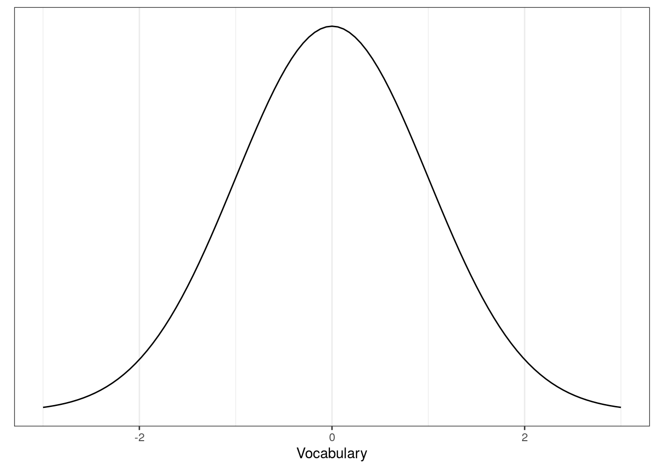
The normal distribution contains two parameters: \(\mu\) and \(\sigma^2\). While \(\mu\) tells us something about where the center is, \(\sigma^2\) gives us information about how spread out the distribution is. Compactly, we write this out as \(\mbox{Normal}(\mu,\sigma^2)\). We can visualize the normal distribution as follows:

To state that data are generated from a normal distribution model, we write:
\[\begin{equation} x_i \sim \mbox{Normal}(\mu,\sigma^2) \tag{2.1} \end{equation}\]
Or equivalently,
\[\begin{equation} x_i \sim \mathcal{N}(\mu,\sigma^2) \tag{2.2} \end{equation}\]