A Introduction to R
In this chapter, we will go over the basics of R.
History of R
R is an open-source programming language for statistical computing and graphics co-created by Ross Ihaka and Robert Gentleman. R is considered a dialect of S, which is also a programming language created by John Chambers and his colleagues at Bell Labs. If you want to find out more about R, check our Roger D. Peng’s website here.
Installation
R works on Mac OS, Windows, and Linux systems. In this section, you will learn how to install R and RStudio, which is an Integrated Development Environment (IDE). You can think of R as a software and RStudio as an add-on to that software. This means R will work without RStudio, but RStudio will not without R!
So why bother installing RStudio then? RStudio has a user-friendly graphical interface that makes working with R less painful. On top of that, RStudio comes equipped with many excellent tools, such as projects, Git integration, etc. Later on, we will try our hands on some of these tools.
To install R, head over to the Comprehensive R Archive Network (CRAN) website, where you will find the most recent version of R for your system.
R: Windows users
Follow the instructions below to install R for a Windows machine:
- Select the ‘Download R for Windows’ link;
- Click on the ‘base’ link;
- Clink on the ‘Download R x.x.x for Windows’ link in the grey box (where x.x.x is the version number);
- Double click on the executable file (.exe) you just downloaded; and
- Follow the on-screen instructions to complete the installation
R: Mac users
Here are the steps you can take to install R for a Mac machine:
- Select the ‘Download R for MacOS’ link;
- Select ‘R-x.x.x.pkg’ under Latest release (where x.x.x is the version number);
- Double on the file icon you just downloaded; and
- Follow the on-screen instructions to complete the installation
RStudio
RStudio can be downloaded from the RStudio website. You should install RStudio Desktop version. Click on the ‘Download’ button.
R and RStudio gets regular updates throughout the year. When you update R and RStudio, you will also need to re-install packages. We can worry about this later! To check for an update in RStudio, go to Help and then Check for updates.
Running RStudio
To get started, launch RStudio. If things work properly, the following interface will show up:
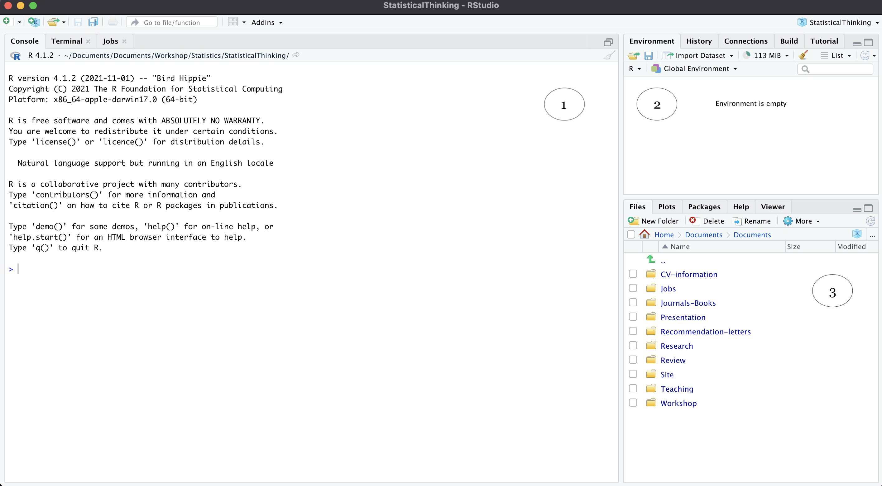
Here, we can see three major panes of the interface. The console (1) is where you input your R codes. The environment tab (2) lists objects we have in our current session, for instance. We will soon see a lot of “things” under the Environment tab when we start working with R. Finally, in 3, the output is where figures are shown. You may also notice that there are many other tabs in (2) and (3). Feel free to click on those to see what they are. As you gain more experience with R, these tabs will become useful. Check them out now to familiarize yourself with the interface of RStudio.
Installing packages
Out of the box, R comes with a lot of useful functions. But to extend existing base R functionality, you can download thousands of R packages published by the R community. Each package consists of a collection of functions and data sets. In this chapter, we will learn how to wrangle data with the help of the dplyr package, which is part of the tidyverse package developed by Hadley Wickham and his colleagues. In fact, the tidyverse package includes several other excellent packages for data science, including ggplot2, readr, and tidyr, just to name a few. Let’s go ahead and install the tidyverse package with the following command:
install.packages("tidyverse") #install.packages("<package_name>")Once the download is complete, load the tidyverse package to make it available in your current R session:
library(tidyverse)You will need to load packages every time you open a new R session. Installation, however, is done once. Note, however, that you will need to re-install packages again when you upgrade R and RStudio.
R as a calculator
One of the most basic ways to use R is as a calculator. The four basic arithmetic operators are:
- addition (+);
- subtraction (-);
- division (/); and
- multiplication (*).
5 + 4 - 2
5 - 4 + 2
5 + 4 * 2
5 / 4 + 2
Spaces are added to make codes human-friendly.
5+4-2is the same as5 + 4 - 2, but the latter is easier to read. As you work your way through R, remember that codes are meant for other humans (or future you) as much as for computers.
The order of operations is PEMDAS (Parentheses, Exponents, Multiplication and Division, and Addition and Subtraction). If you want to override this order, stick parentheses in places where you want them to be evaluated first.
(5 + 4) * 2
(5 + 4) * (2 + 5)
(5 + (4 / 2)) + (2 * 3)
Here are three more operators:
- exponent (^)
- modulus (%%); and
- integer division (%/%)
2 ^ 3
3 ^ 4
5 %% 2
8 %% 3
5 %/% 2
8 %/% 3
Base R has plenty of math functions, some of which are shown below. We will get to know them before long.
sum()
mean()
sd()
min()
max()
log()
sqrt()
exp()
Vector and assignment
Many things in R are objects. Put simply, an object is a “thing” stored in R’s memory. Common objects are vectors, matrices, data frames, lists, and functions. The most basic object is a vector. We can create a vector (or any other objects) with an assignment operator <-. Below, the code length <- 3 means an object named length gets the value of 3.
length <- 3
width  <- 4
size   <- length * width
Object names must start with a letter, and can only contain letters, numbers, _ and .. Generally speaking, object names should be informative (e.g., numbers not n or address not adr). For a longer object name, use snake_case where you separate lowercase words with _ (e.g., city_code not City_Code or CityCode).
Once an object is created, you can inspect its “content” by typing its name. As you type up an object name, RStudio offers auto-completion. Hit Tab to select the name.
length
#> [1] 3

width
#> [1] 4
Pay attention to the output. R tells us that length is a vector of length one (i.e., a vector with one element). The same is true of width.
You can combine multiple elements into a single vector with c() which stands for combine. A colon (:) is another quick way to create a sequence of integers.
numbers <- c(-2, 0, 2, NA, 1, 3, -3)                #NA represents missing data
names   <- c("Jack", "James", "Jill", "Alix")       #characters
answers <- c(TRUE, FALSE, TRUE, TRUE, TRUE, FALSE)  #logicals
num1    <- 1:5                                      #equivalent to c(1, 2, 3, 4, 5)
num2    <- c(1:5, c(12, 16, 19), 30:40)
When an object is no longer needed, you can remove it with rm() function
rm(num1, num2, names)We will use the assignment operation all the time. Soon, you will start typing <- over and over again, and this can be painful. Luckily, RStudio has keyboard shortcuts for the assignment operator:
- Windows: Alt and - (minus sign)
- Mac: Option and -
RStudio automatically surrounds <- with spaces, which again makes codes easy to read. Compare nums<-1:10 with nums <- 1:10. Which one is easier to read? Of course, it’s the latter!
We have created a few objects in this section. If you glance over to the Environment tab, you will find the names of all objects that we have created.
Vectorized operation
For now, we will focus on numeric vectors. Look at the code below, what do you think will happen in num1 + num2?
num1  <- c(1, 4, 12, 8, 6, 5)
num2  <- c(2, 5, 9, 11, 2, 3)
num1 + num2
Arithmetic operations in R are vectorized. That is, an operation is done on all elements of a vector. More concretely, when you instruct R to sum num1 and num2 together, R begins by adding 1 and 2 together, move on to sum the next pair (4 and 5), and on and on and on. Try it in your console to see the results!
Exercises
- Multiply
num2withnum1. What do you get?
num1  <- c(3, 5, 7, 9, 11, 13)
num2 <- c(1, 2)- Divide
num1by3. What do you get?
num1 <- c(3, 5, 7, 9, 11, 13)- Run the following code. What went wrong?
num  <- 10:16
odd  <- c(1, 3, 5)
num * odd
R uses a recycling rule: A shorter vector is expanded to be of the same length as a longer one. We get a warning message in 3 since num has 7 elements while odd has 3. We cannot expand the length of odd to match that of num. But note that R still tries its best to sum the two vectors per our instructions. It’s important that we learn this early on. When we work with data frames, a warning message like this one will be much harder to parse.
Properties
For each vector, we can inspect its type (i.e., what is it?) and length (i.e., how many elements?) with the following functions:
num  <- c(3, 5, 11, 13)
typeof(num)
length(num)
Comparison operators
In R, we can test if one value is greater than, less than, or equal to another value. We can also check if the “content” inside each vector meets our conditions. To do this, we need to talk about relational/comparison operators.
>greater than<less than>=greater than or equal to<=less than or equal to==exactly equal to!=not equal to
5 > 6
11 == 11
12 != 10
The above example may look silly. But once we apply these operators to vectors, we can see how extremely useful they are.
nums  <- c(2, 4, 7, 9, 11, NA)
nums  == 11
nums  != 11
Notice what R prints out with nums == 11. A vector of TRUE and FALSE. This is known as a logical vector.
This whole comparison operations will be of limited use if we have to conduct each “test” one by one. But luckily:
nums >  5  &  nums <  10
nums <= 7  |  nums >  10
nums <= 7  |  nums != 11
nums <= 10 & !(nums %% 2 == 0)
Exercises
- Run the following codes. What are the differences between the two tests?
nums  <- c(2, 4, 7, 9, 11, NA)
nums  <  9
nums <= 9- We can apply these operators to solve some interesting problems. Can you explain what the codes do?
nums  <- c(2, 4, 7, 9, 11, NA)

(nums %% 2) == 0
(nums %% 2) != 0- Go through the codes below. What “results” do you expect to do? Run the code to check our answers.
nums <- c(10, 12, 17, 19, 16, 21, 11, 13, 15, 6, 9, 10)

nums > 5 | nums < 10
nums > 5 & nums < 10
nums == 13 | nums >= 19
nums == 13 & nums >= 19
Indexing and subsetting
In the previous section, we learn how to check if each element inside a vector meets our certain conditions. While this is certainly useful, we may want instead to “extract” certain values from the vector rather than getting a vector of T or F. We can easily do that with subsetting. Let’s begin with subsetting with positive integers.
scores <- c(3, 12, 8, 2, 4, 11, 15, 19, 3, 7, 6, 9)
scores < 7        #or check <- scores < 7

scores[1:2]
scores[c(1, 3, 5)]
scores[[2]]       #get a single element, scale better with lists
We can subset with a comparison function, which will keep values that are TRUE:
scores[scores < 7]

# Obtain position numbers
which(scores < 7)      #then
scores[which(scores < 7)]
R Projects
Before we wrap this chapter, it’s time to talk about our workflow!
- Ideally, we want to keep a record of what we have done in R, so we can recreate everything later;
- Also, we want to run some analyses on our data and save all the results (figures, model outputs, etc.) in one place;
- Later in our career, we may want to share codes with our colleagues or publish our analyses as supplementary materials
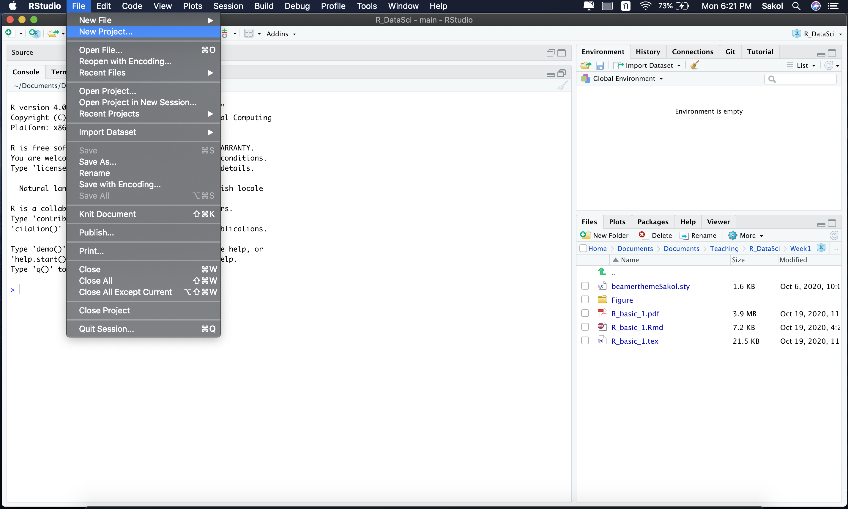
RStudio offers a nice way to achieve all of these goals with R projects. With R projects, seasoned R users can keep all the files associated with a project together in a single “folder”. To create a project from R studio, click File from the top menu and then select New Project.
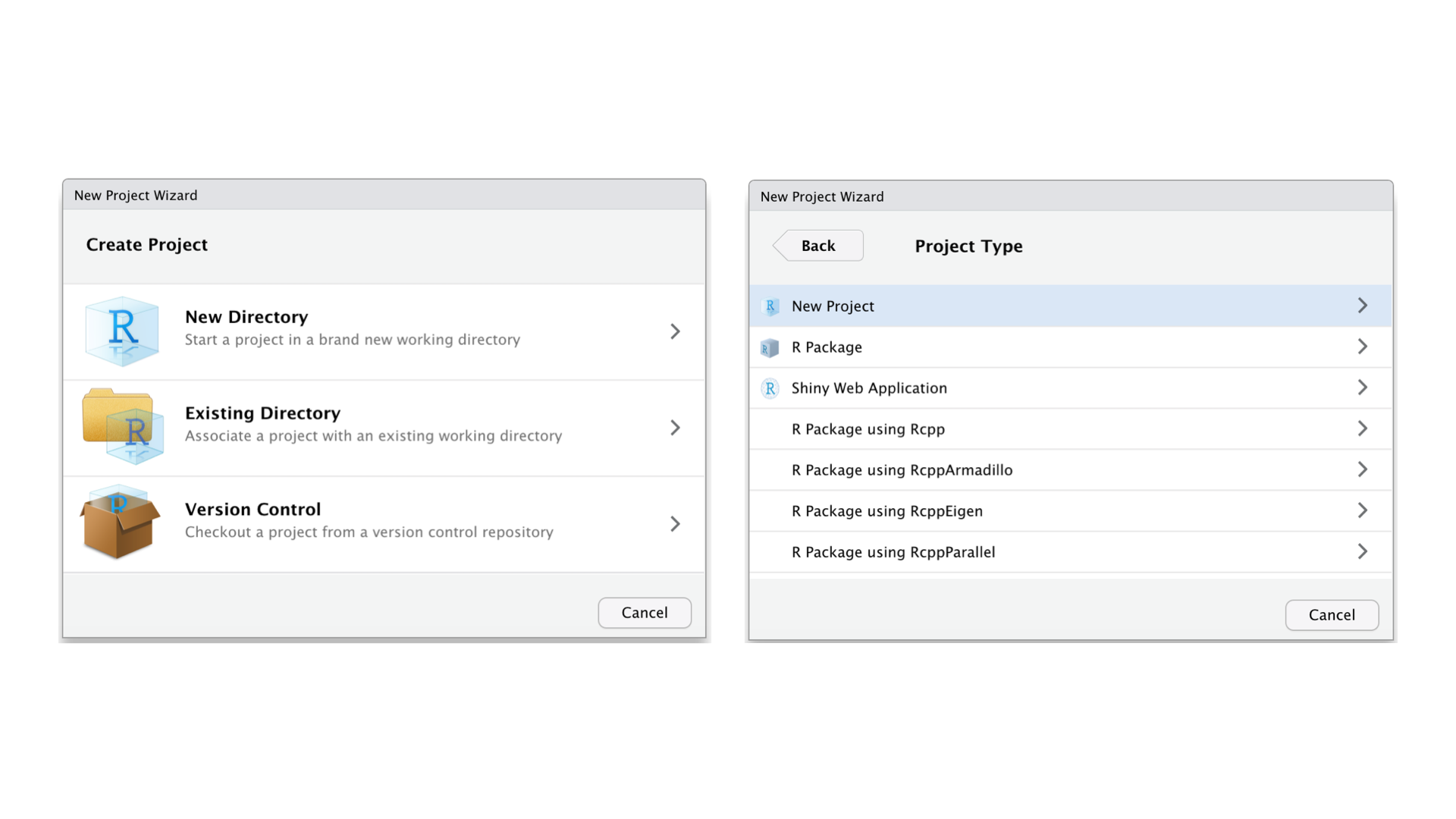
Then, select New Directory and New Project. Provide a directory name (aka a folder name). We can choose to place this newly-created R project in any folder we want by clicking Browse and change a directory.
Once we complete all these steps, a new project will pop up. We can then check where our project lives with the following function:
getwd()Alternatively, we can see our current directory under Console.
At this point, it is worth asking why we need to bother with this? What’s the point of creating a project? Run the following code (adapted from R for Data Science, p. 116) and check your project’s folder:
library(tidyverse)

ggplot(diamonds, aes(carat, price)) +
  geom_point(alpha = 0.2) +
  theme_bw()

ggsave("diamonds.png")

write_csv(diamonds, "diamonds.csv")
But how can we keep track of our analyses? How can we document every step we take to complete a project? The answer to these questions is: R script. An R Script, not the console, should be where your codes live. Click on File from the top menu, then select New File and then R script.
What should you include in an R script? As a general rule, do the following:
- Begin with general comment about your script;
- Then, load all the packages you need in the preamble;
- Use comments to provide context for your analysis;
- Indent your codes and use new lines to your advantage.