Section 4 The Basics of R
Once you understand the basics of R’s data types, some of the more advanced features of R start to make sense.
R is built around a few basic pieces - once you understand them, it’s easier to understand more complex commands, since everything is built from the same basic foundations.
In programming terms, we can refer to the basic pieces that make up R as data types.
4.1 Basic data types
4.1.1 Numbers
The numeric data type allows you to work with numbers. R can do all the basic operations you’d expect: addition, subtraction, multiplication and division.
At the most basic level, you can use R as a calculator by doing
standard operations like +, -, / (division), * (multiplication),
^ (power) on numeric data:
> #addition
> 1 + 1
## [1] 2> #multiplication
> 2.5 * 3## [1] 7.5> #to the power of
> 8^2## [1] 64> #exponentiating
> exp(0.36)## [1] 1.433329> #log transformation
> log10(6.66)## [1] 0.8234742R also has an integer (whole number) data type. Integers (usually) work exactly the same as numeric data, so you don’t need to worry too much about the difference for now. Integers will automatically be converted to the more general numeric format when needed:
# You can specify that data should be integers using "L"
## Addition
2L + 3L
## [1] 5# if we add a decimal place, R will automatically converts the result to numeric
3L + 0.1## [1] 3.14.1.2 Characters (text)
The character data type allows you to store and manipulate
text. Character data is created by wrapping text in either single ' or
double " quotes. In programming terms, we also refer to each chunk of text
as a string:
"apple"## [1] "apple"#we can change it to uppercase
toupper("crab apple")## [1] "CRAB APPLE"# Get part of a string.
substr("apple", 1, 3) #telling it to get the first 3 letters## [1] "app"# Stick multiple strings together with paste0
paste0("crab", "apple")## [1] "crabapple"4.1.3 Factors (categorical data)
Factors are how R represents categorical data. They have a fixed number of levels, that are set up when you first create a factor vector:
severity = sample(c("Moderate", "Severe"), 10, replace=TRUE)
# Setting 'levels' also sets the order of the levels
sev_factor = factor(severity, levels = c("Moderate", "Severe"))
sev_factor
## [1] Moderate Moderate Moderate Moderate Moderate Moderate Severe Severe Moderate Severe
## Levels: Moderate Severe4.1.4 Logical (True/False)
The logical data type is used to represent the True/False result
of a logical test or comparison. These are represented by the
special values of TRUE and FALSE (basically 1 and 0, with special labels
attached to them). To do logical comparisons, you can use syntax like:
==: equals. Note that you need a double equal sign to compare values, a single equal sign does something different.
> "a" == "b"## [1] FALSE<,>: less than, greater than
3 < 4## [1] TRUE<=,>=: less than or equal to, greater than or equal to
10 >= 9## [1] TRUE!=: not equal to
"goodbye" != "spss"## [1] TRUE4.2 Converting between types
Occasionally your data will be read in from a file as the wrong type. You might be able to fix this by changing the way you read in the file, but otherwise you should convert the data to the type that makes the most sense (you might have to clean up some invalid values first).
You will want to check first what variable type your variables have been read in as. We can use the “class” function and select individual variables from the dataset
class(data$sex)## [1] "character"class(data$neuroticism)## [1] "numeric"… or if we want to know it for the whole dataset, we can use the structure function.
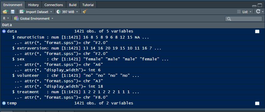
str(data)## tibble [1,421 x 5] (S3: tbl_df/tbl/data.frame)
## $ neuroticism : num [1:1421] 16 8 5 8 9 6 8 12 15 NA ...
## ..- attr(*, "format.spss")= chr "F2.0"
## $ extraversion: num [1:1421] 13 14 16 20 19 15 10 11 16 7 ...
## ..- attr(*, "format.spss")= chr "F2.0"
## $ sex : chr [1:1421] "female" "male" "male" "female" ...
## ..- attr(*, "format.spss")= chr "A6"
## ..- attr(*, "display_width")= int 6
## $ volunteer : chr [1:1421] "no" "no" "no" "no" ...
## ..- attr(*, "format.spss")= chr "A3"
## ..- attr(*, "display_width")= int 18
## $ treatment : num [1:1421] 1 2 2 1 2 2 2 1 1 1 ...
## ..- attr(*, "format.spss")= chr "F8.0"We can also see this for the first variables in the dataframe by clicking the arrow next to our dataframe in the environment.
Data viewer example
If you have data in a format that needs to be changed, for example here, we would like our treatment variable to be a factor, not numeric, we can use functions like as.character(), as.numeric() and as.logical(). These functions will
convert data to the relevant type. Probably the most common type conversion
you’ll have to do is when numeric data gets treated as text and is stored
as character. Numeric operations like addition won’t work until you fix
this:
"1" + 1## Error in "1" + 1: non-numeric argument to binary operatorone_fixed = as.numeric("1")
one_fixed + 1## [1] 2In our dataset we will change our numeric ‘treatment’ variable to a factor, so it can be used as such in subsequent analyses. We will also convert our character vectors to factor.
data$treatment <- as.factor(data$treatment)
data$sex <- as.factor(data$sex)
data$volunteer <- as.factor(data$volunteer)
4.3 Variables: Storing Results
The results of calculations in R can be stored in variables: you give a name to the results, and then when you want to look at, use or change those results later, you access them using the same name.
You assign a value to a variable using either = or <- (these
are mostly equivalent, don’t worry too much about the difference), putting
the variable name on the left hand side and the value on the right.
NOTE THAT EVERYTHING ON THE RIGHT HAND SIDE IS BEING ASSIGNED TO THE NAME YOU GIVE ON THE LEFT
data$personality_total <- data$neuroticism + data$extraversion
# Accessing saved results
#data$personality_total
This variable will have also now saved into your dataframe:
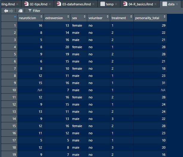
Data viewer example
# Using saved results in another calculation
data$severe_personality = data$personality_total >= 20
#data$severe_personality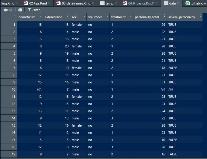
Data viewer example
# Changing a variable: this will overwrite the old value with the
#   new one, the old value won't be available unless you've
#   stored it somewhere else, or named the new variable something different
data$personality_total <- data$personality_total + 2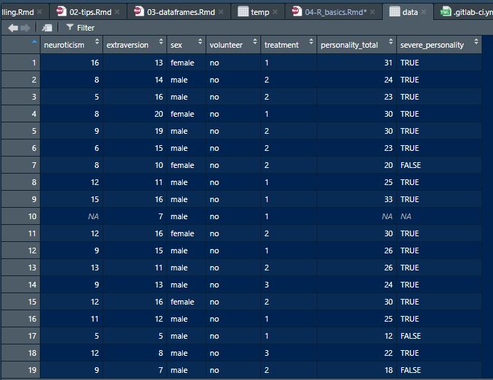
Data viewer example
Now our personality total variable is not the same as our original one, it has been overwritten with our new command.
When you assign a variable, you’re asking R to remember some data so you can use it later. Understanding that simple principle will take you a long way in R programming.
Variable names in R should start with a letter (a-zA-Z), and
can contain letters, numbers, underscores _ and periods ., so
model3, get.scores, ANX_total are all valid variable names.
4.3.1 Missing values
Some of you smart cookies may have noticed that our ‘personality_total’ variable has some NAs…
Functions like sum() and mean() will produce a missing
result by default if any values in the input are missing. Use the
na.rm = TRUE option (short for “NA remove”) to ignore the missing values
and just use the values that are available:
mean(data$neuroticism)## [1] NAmean(data$neuroticism, na.rm = TRUE)## [1] 11.46888If we wanted to re-make our personality_total variable so that individuals with values for only one of the two personality variables are assigned that value as their total (we probably wouldn’t want to do this, but let’s say we do!):
data$personality_total <- rowSums(cbind(data$neuroticism, data$extraversion), na.rm = TRUE)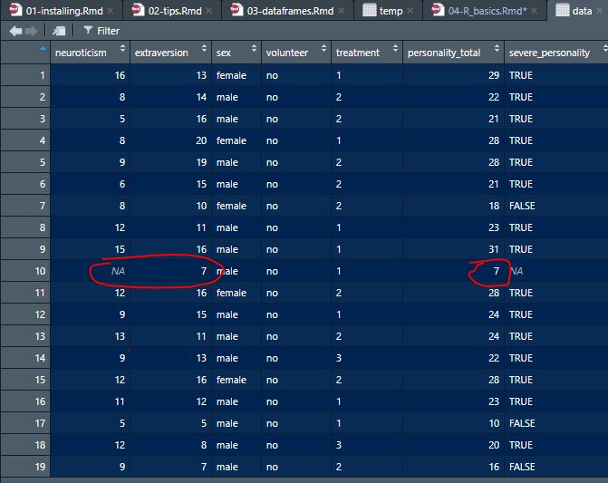
Data viewer example
Other functions in R will automatically remove missing values, but will usually warn you when they do. It’s always good to check how missing values are being treated, whatever tool you’re using.