Section 1 Getting started with R
1.1 Installing R
R, on its own, is basically just a command-line: you send it commands and it sends back output. It comes with a “GUI” (graphical user interface), but it’s pretty ugly and we wouldn’t recommend it.
To install R, go to the CRAN website and click the download link for either Windows or Mac OS X.
1.1.1 Windows instructions
- Click Download R for Windows
- Click
"base", and download. - Run the installer and install - you shouldn’t need to change any of the options.
1.1.2 Mac OS X instructions
- Click Download R for (Mac) OS X
- Download the
.pkgfile for the latest release - Open the installer and go through it:
- “Install for all users” (the default) should be fine (if you have install rights on your machine)
1.2 Installing RStudio
It’s best to work with R through RStudio: it’s a nice interface that makes it easy to save and run scripts, and see all the output and plots presented in the same window.
Head to the RStudio website to download the free version of RStudio Desktop: the free version is 100% fine and isn’t missing any important features.
1.3 Running RStudio
Open up RStudio and you should see the standard 4-pane layout:
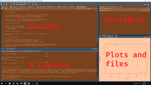
This may look like information overload at first, but most of the time, you’ll just be looking at the “Scripts” section where you’ve written your code.
Optional: Go to Tools -> Global options -> Appearance and switch to a dark theme - it’s easier on the eyes and it looks cool.
You should now be able to run your first R command
by clicking in the console and typing 1 + 1 and hitting
<Enter>:
1 + 1## [1] 21.4 Working directories
Wherever your working directory is, your files will save to. If you want to call in files from/save files to a different folder, you will need to specify an alternative filepath. For this reason, you should set your working directory to a convenient location at the start of each session.
getwd() #to see where your current working directory is
setwd("C://Users//sode2138//OneDrive - The University of Sydney (Staff)") #to set your working directory
For ease, we will use Rstudio’s point-and-click capabilities to set your working directory. In the toolbar at the top of the scripts section, navigate to “session” and scroll down to “set working directory,” then “choose working directory.” From here, choose the folder that you want to read and save your files to today.
Having all your files in one folder and setting this as your working directory will mean the difference between having to write:
data = haven::read_spss("C://Users//sode2138//OneDrive - The University of Sydney (Staff//Personality.sav")And:
data = haven::read_spss("Personality.sav")1.5 Using scripts
We just ran some code in the console. BUT NO-ONE DOES THIS IN REAL LIFE.
It’s best to put every step of your data cleaning and analysis in a script that you save, rather than making temporary changes in the console.
Ideally, this will mean that you (or anyone else) can run the script from top to bottom, and get the same results every time, i.e. they’re reproducible.
To open a new script, click File > New File > R script.
1.5.1 Script layout
Most R scripts I write have the same basic layout:
- Loading the libraries I’m using
- Loading the data
- Changing or analysing the data
- Saving the results or the recoded data file
For a larger project, it’s good to create multiple different scripts for each stage, e.g. one file to recode the data, one to run the analyses.
When saving the recoded data, it’s best to save it as a different file - you keep the raw data, and you can recreate the recoded data exactly by rerunning your script.
R won’t overwrite your data files when you change your data, unless you specifically ask it to. When you load a file into R, it lives in R’s ‘short-term memory,’ and doesn’t maintain any connection to the file on disk. It’s only when you explicitly save to a file that those changes become permanent.
1.5.2 Saving your scripts
Save your script (to your current working directory) by clicking the save icon, or File>Save. You will be prompted to give your script a name the first time you do this. Once saved, you will see the script appear in the bottom right pane displaying all of the files within your working directory.
1.6 Installing your first packages
A lot of the most useful tools in R come from third-party packages. Thankfully
they’re easy to install, through the install.packages() command. We only need
to install a package on our computer once, but we need to load it every time we
start a new session using the library() command. We will install and load some
packages to use in today’s workshop:
install.packages("tidyverse") #install
install.packages("dplyr")
install.packages("haven")
install.packages("psych")

library(tidyverse) #load packages
library(dplyr)
library(haven)
library(psych)
The install process should be automatic, and it will also install other packages
that your package needs. Just in case, you should check the last few lines of
the output that install.packages() produces, and look for messages like:
package ‘tidyverse’ successfully unpacked and MD5 sums checked