Section 6 Example data cleaning and manipulation; Example descriptive statistics
Now that we’ve covered the fundamentals of R, we can go through an example to see everything works in practice.
We’ll use an example dataset from the carData package, a study
looking at personality and how it relates to people’s decision to volunteer
as a research participant.
We’ve already loaded this in under the name ‘data.’
We’ll run through some different steps, working towards some simple analyses
of the data. In this format, the steps will be broken up in different chunks,
but normally they would all be saved in a single script which could
be run in one go. In a script, it can be useful to label each
section with a commented heading - if you end a comment line with at least 4 #’s,
RStudio automatically treats it as a heading, and you’ll be able to jump
to that section:
### Load libraries #####
# Code goes here

### Load data ##########
# More code here
6.1 Loading libraries
The first step in any analyses is to load any libraries we’re going to use. If you’re part way through an analysis and realise you’re going to use another library, go back and add it to the top of the script.
6.2 Loading data
We already did this step using:
data = haven::read_spss("Personality.sav")Let’s check the format of the data using str() again, short for structure:
str(data)## tibble [1,421 x 7] (S3: tbl_df/tbl/data.frame)
## $ neuroticism : num [1:1421] 16 8 5 8 9 6 8 12 15 NA ...
## ..- attr(*, "format.spss")= chr "F2.0"
## $ extraversion : num [1:1421] 13 14 16 20 19 15 10 11 16 7 ...
## ..- attr(*, "format.spss")= chr "F2.0"
## $ sex : Factor w/ 2 levels "female","male": 1 2 2 1 2 2 1 2 2 2 ...
## $ volunteer : Factor w/ 2 levels "no","yes": 1 1 1 1 1 1 1 1 1 1 ...
## $ treatment : Factor w/ 3 levels "1","2","3": 1 2 2 1 2 2 2 1 1 1 ...
## $ personality_total : num [1:1421] 29 22 21 28 28 21 18 23 31 7 ...
## $ severe_personality: logi [1:1421] TRUE TRUE TRUE TRUE TRUE TRUE ...All the columns have a sensible format here: the three personality scores are integers (whole numbers), the three categorical variables are factors, and the severe personality variable is a logical (true/false). If you need to change the type of any variables in your data, it’s best to do it right after loading the data, so you can work with consistent types from that point on.
6.3 Recoding
Let’s go through some basic recoding. First we’ll create a variable to show whether someone is above or below the mean for extraversion. We’ll do this manually first, using the tools we’ve covered so far:
# Create a vector that's all "Low" to start with
data$high_extraversion = "Low"
# Replace the values where extraversion is high
data$high_extraversion[data$extraversion > mean(data$extraversion)] = "High"
# Make it a factor
data$high_extraversion = factor(
    data$high_extraversion,
    levels = c("Low", "High")
)
Next we’ll code people as either “introverts” or “extroverts” based
on their scores. We’ll use functions called mutate() and case_when() to do this, which makes the process we carried out above a bit more automatic.
It will also handle missing values better than our simple manual procedure, leaving missing scores missing in the result.
data <- mutate(data, personality_type =
case_when(extraversion > neuroticism ~ "Extravert",
    extraversion < neuroticism ~ "Introvert"))


# Make it a factor
data$personality_type = factor(
    data$personality_type,
    levels = c("Introvert", "Extravert")
)
mutate() and case_when() make it easy to create
a vector based on logical arguments (e.g., greater (>) or less (<) than; equal to (==), not equal to (!=) etc…)
We’ll also code neuroticism as either “low” or “high” based on whether it’s above the mean (N.b., remember there are missing values in neuroticism, so we must include that as an argument when using the mean() function)::
data <- mutate(data, high_neuroticism =
case_when(neuroticism > mean(neuroticism, na.rm = TRUE) ~ "High",
      neuroticism <= mean(neuroticism, na.rm = TRUE) ~ "Low"))

data$high_neuroticism = factor(
    data$high_neuroticism,
    levels = c("Low", "High")
)
Since the example dataset we’re using doesn’t have quite enough variables, let’s also create a new one, a score on a depression scale similar to PHQ-9:
# Advanced code: run this but don't worry too much about what
#   it's doing
set.seed(1)
data$depression = round(
  19 +
  0.5 * data$neuroticism +
  -0.8 * data$extraversion +
  0.5 * (data$sex == "female") +
  rnorm(nrow(data), sd = 3)
)
We’ll recode this depression score into categories using
cut(), which allows us to divide up scores into
more than two categories:
data$depression_diagnosis = cut(
    data$depression,
    breaks = c(0, 20, 25, 33),
    labels = c("None", "Mild", "Severe"),
    include.lowest = TRUE
)
6.4 Descriptive Statistics
Before doing any actual analysis it’s always good to use descriptive statistics to look at the data and get a sense of what each variable looks like.
6.4.1 Quick data summary
You can get a good overview of the entire dataset using
summary():
summary(data)## neuroticism extraversion sex volunteer treatment personality_total severe_personality high_extraversion
## Min. : 0.00 Min. : 2.00 female:780 no :824 1:329 Min. : 6.00 Mode :logical Low :691
## 1st Qu.: 8.00 1st Qu.:10.00 male :641 yes:597 2:710 1st Qu.:20.00 FALSE:317 High:730
## Median :11.00 Median :13.00 3:382 Median :24.00 TRUE :1097
## Mean :11.47 Mean :12.37 Mean :23.79 NA's :7
## 3rd Qu.:15.00 3rd Qu.:15.00 3rd Qu.:28.00
## Max. :24.00 Max. :23.00 Max. :40.00
## NA's :7
## personality_type high_neuroticism depression depression_diagnosis
## Introvert:563 Low :719 Min. : 0.00 None :1191
## Extravert:756 High:695 1st Qu.:12.00 Mild : 193
## NA's :102 NA's: 7 Median :15.00 Severe: 30
## Mean :15.06 NA's : 7
## 3rd Qu.:18.00
## Max. :33.00
## NA's :76.4.2 Frequency tables
You can count frequencies of categorical variables with
table():
table(data$sex)##
## female male
## 780 641table(data$sex, data$volunteer)##
## no yes
## female 431 349
## male 393 2486.4.3 Histograms: distributions of continuous variables
Histograms are good for checking the range of scores
for a continuous variable to see if there are any
issues like skew, outlying scores etc.. Use hist()
to plot the histogram for a variable:
hist(data$neuroticism)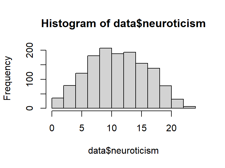
6.4.4 Scatterplots: relationship between two continuous variables
Scatterplots are useful for getting a sense of whether or
not there’s a relationship between two continuous variables.
The basic plot() function in R is quite flexible, so to
produce a scatter plot we just give it the two variables
and use type = 'p' to indicate we want to plot points.
plot(data$neuroticism, data$depression, type='p')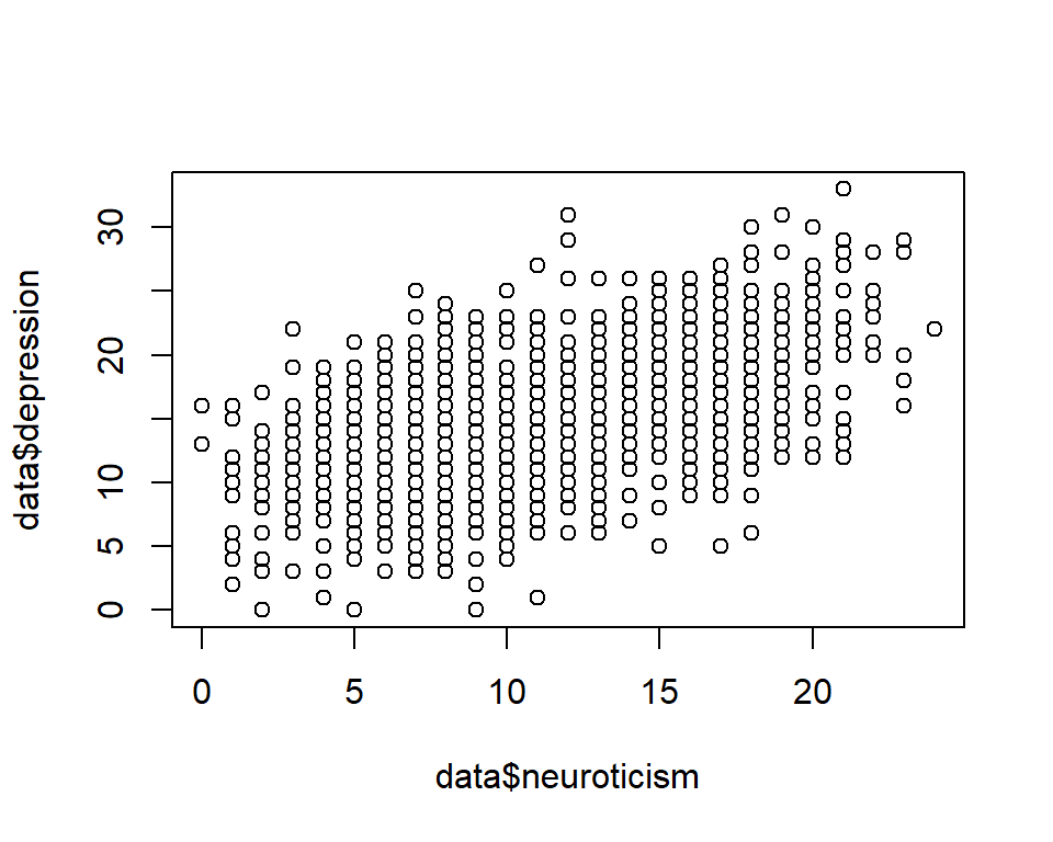
This plot doesn’t look great - we’ll cover ways to produce
better plots in future sessions. But you can see there’s a positive
correlation between neuroticism and depression.[^fakedata]
To check the correlation we can use cor():
cor(data$neuroticism, data$depression, use="complete.obs")## [1] 0.5346548