7 Regression models
7.1 Introduction
For regression analysis to be performed, data has to be stationary. Or the equation has to be rewritten in such a form that indicates a relationship among stationary variables.
What is stationary? Stationarity refers to a situation where the underlying stochastic process that generates the data is invariant with respect to time. On the other hand, if the characteristics over the time changes we call it a non-stationary process.
Now the obvious question is what are the characteristics that has to be invariant? We can list it in the following manner: mean variance covariance etc
If a series is stationary then we can model it via an equation with fixed coefficents estimated from the past data.
7.2 Conditions for Stationarity
Let us assume a stochastic time series \(y_1, y_2, ...... y_T\) where there are T observations. Now a stochastic process is weakly stationary if
 * $E(y_t)$ is independent of $t$
 * $Var(y_t)$ is not only independent of $t$ but also constant
 * $Covar(y_t, y_s)$ depends on $(t-s)$ but not on $t$ or $s$
Now let us elaborate on the whole issue:
\(E(y_t)\) is independent of \(t\)
What it means is that a stationary series must have a constant mean. That is it should revert back to the mean. It many wonder around here and there but it should have an tendency to come back to the mean. That means the series should show certain amount of randomness around its mean with respect to time.
This also implies that expected value will be the same in each time period. Is that true? Think about a stationary time series: change in the stock prices. Does this mean that expected change in the stock price will be the same in each time period? Is this a realistic thing to expect?
Let’s take a look into an example which might generate stable series:
An AR(1) process:
\[y_t=\alpha+\beta_1*y_{t-1}+e_t \]
If the process has to be stationary then we should have \[\begin{align*} E(y_t)&=E(y_{t-1}) \\ E(y_t)&=\alpha+\beta_1 \times E(y_{t-1})\\ E(y_t)-\beta_1 \times E(y_{t-1})&=\alpha \\ E(y_t)-\beta_1 \times E(y_t)&=\alpha \qquad [since~ E(y_t)=E(y_{t-1})] \\ E(y_t)&=\frac{\alpha}{1-\beta_1} \end{align*}\]
It says that a stable mean requires that \(\beta_1\) must be less than 1, that \[\beta_1 <1\]. Not sure why it says that. What does that mean to be stable? Need to have further elaboration.
\(Var(y_t)\) is a constant and independent of \(t\)
Usually exchange rate and stock prices tend to have an non-constant variance.
\(Cov(y_t, y_s)\) depends on \((t-s)\) but not on \(t\) or \(s\)
This means that covariance depends on the time difference of observation, not the actual time period they are observed. For example, \(Cov(y_1, y_4)=Cov(y_{12}, y_{15})\) because they are both three time periods apart.
A stationary series is also considered to be integrated of order zero. Because it has to be differenced zero times.A non-stationary series is integrated of order \(d\). That means it has to be differenced \(d\) times to make a series stationary. It is usually common to find macroeconomic data to integrated of order(1). That is macroeconomic time-series like GDP, Investment, exports are non-stationary.
7.3 Spurious Regression
In a famous paper, Granger and Newbold(1974) introduced the notion of Spurious Regression. They are the one who first warned that macroeconomic regression has highly autocorrelated residual. That means regression are violating assumptions of no autocorrelations.
In this situation, statistical inference goes haywire. We usually find statistically significant relationship among variables. For example, we might find inflation is affected by temperature and that is statistically significant which is totally absurd.
In general,regression involving two integrated time series of the same order yields significant relationship which is called spurious regression. This is characterized by high \(R^2\), significant \(t\) but this has no meaning. But this does not apply to cointegration which is a special case. We will elaborate on this later.
A spurious regression is like this:
\[y_t=\alpha+\beta_1 x_t+ \epsilon_t\]
Here \(y_t\) and \(x_t\) are both integrated time series. In this situation, the formula of OLS estimator \(\beta_1\) in the denominator has \(\frac{\sum_{i=1}^{n}{(x^2-\bar{x})}}{T}\) or \(\sum_{i=1}^{n}{(x^2-\bar{x})}/T\) does not converge to any limiting value. As a result OLS estimators are not consistent and as a result usual inference procedure becomes invalid.
In a Monte Carlo study, Granger and Newbold(1974), created two non-staionary random walks \(y_t\) and \(x_t\) that were uncorrelated with each other. Then they regressed \(y_t\) on \(x_t\) and found that in the 75 percent of the cases, there is significant relationship.
That means in the 75 percent of the cases a spurious relationship was found. Then Granger and Newbold(1974) concluded that such regressions are characterized by high \(R^2\), low DW statistics and the t-stats are misleading.
Phillips(1986) provided the theoretical proof of the Granger and Newbold experiment. The initial solution to this problem was to first difference. But eventually researchers looked for alternative methods. They first look for cointegration between \(y\) and \(x\).
The first difference form of the regression would be: \[\Delta y_t=\alpha_1+\beta_1 y_t+v_t\] \[where \quad v_t=\epsilon_t-\epsilon_{t-1}\]
It says that if the original error is not serially correlated then the differenced error \(v_t\) is MA(1). I have to check later how this is possible. Anyway, in this case OLS is unbiased but inefficient. This is due to the new error being MA(1).Granger and Newbold(1974)further showed that it does not distort hypothesis testing. Meaning hypothesis testing still owrks.
The strong message here is that we should take great care using non-stationary time series in levels. Then it says that the real message is that we cannot conduct inference unless we detrend the data. Now at this point I get a little confused. Why suddenly detrending gets important? May be the following analysis will shed some light.
7.4 Statistical properties of regression
It has been already established that statiscal properties of OLS hold only when the underlying stochastic process is stationary. Data is stationary or the stochastic process is stationary? Are they the same thing? Data is realization of one particular instance of the underlying stochastic process. Then how they are the same?
Trends in time series can be classified as stochastic or deterministic. We may consider a trend to be stochastic when it shows inexplicable changes in direction We attribute apparent transient trends to high serial correlation with random error The meaning of above statement is that the trend we see in the data is actually not deterministic, it is actually stochastic because it was generated from high serial correlation in random error component
Now it says that data must have the trend removed before they can be used. There are two common approaches to this:
-detrending using a time trend or some deterministic function of time - using differences
Question is which approach is the best?
It depends on the source of non-stationarity. If the non-stationarity stems from the trending pattern, then obviously we should go for detrending with a time trend.
On the other hand, if non-stationarity stems from stochastic or random behaviour then obviously the first approach will not work. In that case, the differncing has to be employed.
7.4.1 Deterministic Trends
We assume that the process is driven by a deterministic trend. Why the term deterministic? Deterministic here probably means there is a specific pattern to it. It addition to deterministic trend, there is also a random component to it. It it’s a linear trend, then it’s easy to take care. Let’s start with a generic expression:
\[y_t=f(t)+ \epsilon_t \] \[ \epsilon_t \sim iid(0,\sigma^2)\] Now if we consider a linear trend, then
\[y_t= \alpha+\beta* t+ \epsilon_t \]
The least square residual from the above equation is a detrended stationary series which can be used in the regression analysis.
\[\hat{\epsilon}_t=y_t-\hat{\alpha}-\hat{\beta}t\]
Time series that can detrended in this manner is called (TSP).
But there is another type of non-stationarity which simply does not go away with detrending. This is the type of non-stationarity that was mentioned by Granger and Newbold (1974). If we still detrend it and use in the regression, it does not help actually. It is called stochastic trending behaviour.
Integrated process that was mentioned in Granger and Newbold(1974) display stochastic trend.
7.4.2 Stochastic Trend
A very common model which shows stochastic trend is random walk model.
\[y_t = \alpha+y_{t-1}+\epsilon_t\]
\[where \quad \epsilon_t \sim iid(0,\sigma^2)\]
By direct substitution, we get \[\begin{align*} y_{t-1}&=\alpha+y_{t-2}+\epsilon_{t-1} \\ y_t&=\alpha+y_{t-1}+\epsilon_t \\ \mbox{Now we can put the value of } y_{t-1} \mbox{ in the above equation}\\ y_t&=\alpha+\alpha+y_{t-2}+\epsilon_{t-1}+\epsilon_t \\ &=\alpha \cdot 2+y_{t-2}+\epsilon_{t-1}+\epsilon_t \\ &=\alpha \cdot 3+y_{t-3}+\epsilon_{t-2}+\epsilon_{t-1}+\epsilon_t \\ &=\sum_{i=0}^\infty(\alpha+\epsilon_{t-i}) \end{align*}\]
That means random walk process is essentially infinite sum of random variables with a non-zero mean. What is this non-zero mean?
\[E(y_t)=t\alpha \quad where \quad E(\epsilon_{t-i})=0\]
We clearly see that the mean depends on \(t\), so it is non-staionary. This series can be turned into stationary process by simply taking the first difference. Then
\[y_t-y_{t-1}=\alpha+\epsilon_t \]
The L.H.S is clearly stationary since it is composed of only a constant and a random component. A series which can be tunred into stationary by differencing is called I(1) or difference stationary process (DSP).
Problem is that TSP and DSP can behave in the same manner. So it is difficult to know which is the underlying fact. That is why it might be difficult to say it from the visual inspection.
Tracing the DSP and TSP process
DSP: \[\begin{align*} y_1=y_0+\beta+\epsilon_1 \\ y_2=y_1+beta+\epsilon_2 \\ =y_0+2*beta+\epsilon_1+\epsilon_2 \\ \vdots \\ y_t=y_0+\beta*t+\epsilon_1+\epsilon_2+\ldots+\epsilon_t \\ \mbox{We can write the above equation in the following form:} \\ y_t=y_0+\beta t+v_t \\ where \quad v_t=\sum_{i=1}^{t}\epsilon_t \end{align*}\]
TSP: \[\begin{align*} y_t=\alpha+\beta*t+\epsilon_t \\ \mbox{We start from t=0} \\ y_0=\alpha+\beta*0+\epsilon_0 \\ =\alpha+\epsilon_0 \\ y_1=\alpha+\beta*1+\epsilon_1 \\ =\alpha+\beta+\epsilon_1 \\ = y_0 -\epsilon_0+\beta+\epsilon_1 \\ y_2=\alpha+\beta*2+\epsilon_2 \\ =y_0-\epsilon_0+\beta*2+\epsilon_2 \\ \vdots \\ y_t=y_0+\beta t+\epsilon_t \quad assuming \quad \epsilon_0=0 \end{align*}\] So, what we get is this: \ on the other hand, \So the difference stems from the error component. In DSP, the error component is non-stationary since \(var(v_t)=\sigma^2t\). This example clearly shows that if we treat DSP as TSP, then we run into problem. This happens because in TSP, we use the residual but if it is DSP, then it remains non-stationary.
7.4.3 Time series Regression
In this lesson, various regression models are studied that are suitable for a time series analysis of data that contains deterministic trends and regular seasonal changes
We first look at linear models for trends
Then we introduce regression models that account for seasonal variation using indicator and harmonic variables
Regression models can also include explanatory variables
The logarithmic transformation, which is often used to stabilise variance, is also considered
Difference from standard regression
Time series regression usually differs from a standard regression analysis because the residuals themselves form a time series
Therefore residuals tend to be serially correlated
When this correlation is positive, the estimated standard errors will be biased, will tend to be less than their true value
Low standard errors will lead to high value of t-statistics and as a result high statistical significance will be attributed
Estimation process
Therefore, correct statistical evidence is important
For example, an environmental protection group can be accused of falsely claiming statistically significant trends.
In this lesson, generalized least squares is used to obtain improved estimates of the standard error to account for autocorrelation in the residual series.
Linear Models
Definition
A model for a time series \({x_t:t=1,\ldots n}\) is linear if it can be expressed as
\[x_t=\alpha_0 + \alpha_1u_{1,t}+\alpha_2u_{2,t}+\ldots+\alpha_mu_{m,t}+z_t\]
Here \(u_{i,t}\) is the value of the \(i\)th predictor (or explanatory) variable at time \(t\) \((i=1,\ldots,m;t=1,\ldots,n)\)
\(z_t\) is error at time \(t\)
\(\alpha_0,\alpha_1,\ldots,\alpha_m\) are model parameters which can be estimated by least squares
Errors from a time series \({z_t}\) with mean 0, that does not have to be Gaussian or white noise
An example of a linear model is the \(p\)th-order polynomial function of t:
\[x_t=\alpha_0+\alpha_1t+\alpha_2t^2+\ldots+\alpha_pt^p+z_t\]
Simple case
A simple special case of a linear model is the straight line model obtained by putting \(p=1\) \[x_t=\alpha_0+\alpha_1t+z_t\] In this case, the value of the line at time \(t\) is the trend \(m_t\)
For more general polynomial, the trend at time \(t\) is the value of the underlying polynomial evaluated at time \(t\)
\[m_t=\alpha_0+\alpha_1t+\alpha_2t^2+\ldots+\alpha_pt^p\]
Many non-linear models can be transformed to linear models. For example, the model \[x_t=e^{\alpha_0+\alpha_1t+z_t}\]
This series \({x_t}\) can be transformed by taking natural logarithms: \[y_t=log(x_t)=\alpha_0+\alpha_1t+z_t\]
Standard least square regression could then be used to fit a linear model and make predictions for \(y_t\)
To make predictions for \(x_t\), the inverse transform needs to be applied to \(y_t\) which in this example is \(exp(y_t)\)
However this usually has the effect of biasing the forecasts of mean values and we discuss correction factors
Stationarity
Linear models for time series are non-stationary when they include functions of time
Differencing can often transform a non-stationary series with a deterministic trend to stationary series
Suppose this is our model \[x_t=\alpha_0+\alpha_1t+z_t\]
then first order differences are given by:
\[\bigtriangledown x_t=x_t-x_{t-1}=z_t-z_{t-1}+\alpha_1\]
Assuming the error series \({z_t}\) is stationary
the series \({\bigtriangledown x_t}\) is stationary as it is not a function of \(t\)
Previously we have found that first-order differencing can transform a non-stationary series with a stochastic trend to a stationary series
For example, random walk, the first difference makes it stationary series
Differencing can remove both stochastic and deterministic trends from time series
If the underlying trend is a polynomial or order \(m\), then \(m\)th-order differencing is required to remove the trend
Differencing the straight-line function plus white noise leads to a different stationary time series compared to the one we can by subtracting the trend.
When we subtract the trend it gives white noise
When we difference, it gives rise to consecutive white noise terms which is an example of an MA process
** Simulation **
In a time series, it is common for the error series \({z_t}\) in equation to be autocorrelated
In the code below, a time series with an increasing staright line trend \(50+3t\) with autocorrelated errors is simulated and plotted:
set.seed(1)
z  <- w  <-  rnorm(100, sd=20)
for (t in 2:100)  z[t]  <- 0.8*z[t-1]+w[t]
Time  <- 1:100
x  <- 50 + 3*Time +z
plot(x,xlab="time", type="l")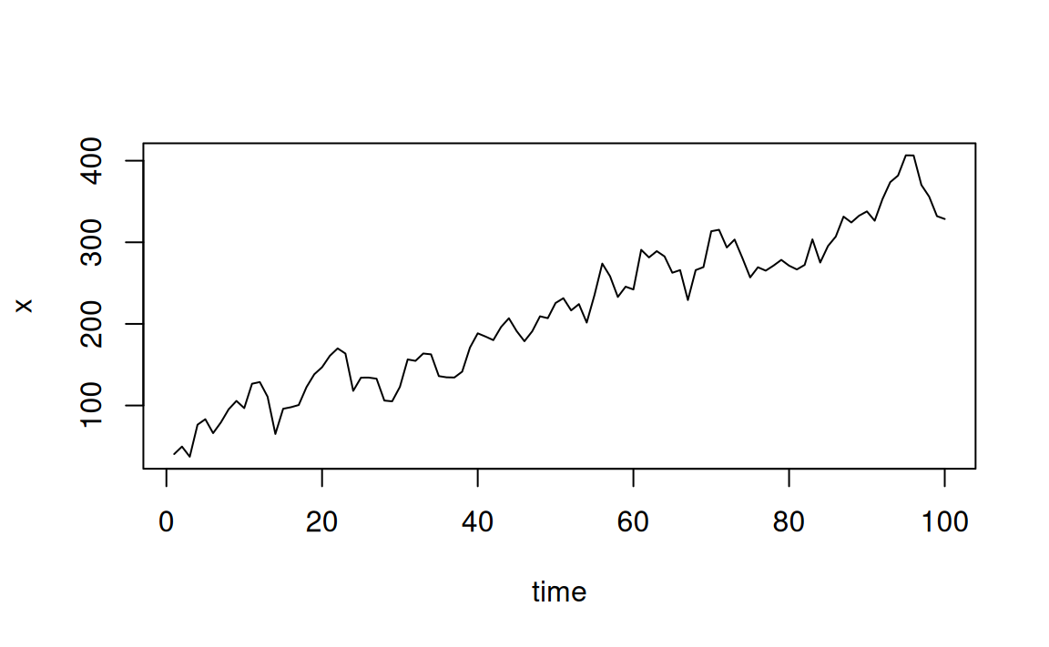
The model for the code above can be expressed as \(x_t=50+3t+z_t\) where \({z_t}\) is the \(AR(1)\) process \(z_t=0.8z_{t-1}+w_t\) and \(w_t\) is Gaussian white noise with \(\sigma=20\)
Fitted models
Model fitted to simulated data
Linear models are usually fitted by minimising the sum of squared errors
\(\sum{z_{t}^{2}}=\sum{(x_t-\alpha_0-\alpha_1u_{1,t}-\ldots-\alpha_mu_{m,t})}^2\)
x.lm <- lm(x ~ Time)
coef(x.lm)
sqrt(diag(vcov(x.lm)))
In the code above, the estimated parameters of the linear model are extracted using coef.
Note that estimates are close to underlying parameter values of 50 for the intercept and 3 for the slope
The standard errors are extracted using the square root of the diagonal elements obtained from vcov
These standard errors are to be underestimated because of autocorrelation in the residuals.
The function summary can also be used to obtain this information but tends to give additional information
For example t-tests, which may be incorrect for a time series regression analysis due to autocorrelation in the residuals
After fitting a regression model, we should consider various diagnostics plots
In the case of time series regression, an important diagnostic plot is the correlogram of the residuals:
acf(resid(x.lm))
pacf(resid(x.lm))
As expected, the residual time series is autocorrelated
We find lag 1 partial autocorrelation is significant, which suggests that the residual series follows an AR(1) process.
This is expected given that an AR(1) process was used to simulate these residuals
Model fitted to temperature series (1970-2005)
 www <-"./RAWDATA/itsr_data/global.dat"
 Global <- scan(www)
 Global.ts <- ts(Global, st = c(1856, 1), end = c(2005,
12), fr = 12)
 temp <- window(Global.ts, start = 1970)
 temp.lm <- lm(temp ~ time(temp))
 coef(temp.lm)
Now let’s find the confidence interval
confint(temp.lm)The confidence interval for the slope does not contain zero, which provide statistical evidence of an increasing trend in global temperatures if the autocorrelation in the residuals is negligible.
However, the residual series is positively autocorrelated at shorter lags, this is evident in the following acf plot, leading to an underestimate of the standard error and too narrow a confidence interval for the slope
Bur first let’s just draw the residual series
plot(x=time(temp), y=resid(temp.lm), type='l')Then let’s find the acf
acf(resid(lm(temp ~ time(temp))))Then let’s find the pacf
pacf(resid(lm(temp ~ time(temp))))PACF may indicate AR(2)
7.5 Generalised least square (GLS)
We have seen that in time series regression it is common and expected that the residual series will be autocorrelated
For a positive serial correlation in the resdiual series, this implies that the standard errors of the estimated regression parameters are likely to be underestimated and should therefore be corrected.
A fitting procedure known as generalized least square (GLS) can be used to provide better estimates of the standard errors of the regression parameters to account for the autocorrelation in the residual series
The procedure is essentially based on maximizing the likelihood given the autocorrelation in the data and is implemented in R in the gls function within the \(nlme\) library
7.5.1 GLS fit to simulated series
7.5.2 Fitting simulated data
The following example illustrates how to fit a regression model to the simulated series
library(nlme)
x.gls  <- gls(x ~ Time, cor=corAR1(0.8))
coef(x.gls)
sqrt(diag(vcov(x.gls)))
A lag 1 autocorrelation of 0.8 is used above because this value was used to simulate the data. Since we have simulated data, we already knew the data generating process.
But in real life, we will have historial data. Hence we will have to first estimate the coefficient from the residuals.
This value will be estimated from the correlogram of the residuals of a fitted linear model
The parameter estimates from GLS will generally be slightly different from those obtained with OLS.
The slope is estimated as 3.06 using lm but 3.04 using gls
In principle GLS estimators are preferable because they have smaller standard errors
Temperature data
Let’s calculate an approximate 95% confidence interval for the trend in the global temperature series (1970 - 2005)
GLS is used to estimate the standard error accounting for the autocorrelation in the residual series
In the gls funcdtion, the residual series is approximated as an AR(1) process with lag 1 autocorrelation of 0.7 read from figure
temp.gls <- gls(temp ~ time(temp), cor = corAR1(0.7))
confint(temp.gls)
The confidence interval above are now wider than they were previously
Zero is not contained in the intervals
This implies that the estimates are statistically signficant
That means the trend is significant
Thus there is statistical evidence of an increasing trend in global temperatures over the period 1970-2005
If the current condition persists, temperatures may be expected to continue to rise in the future
7.5.3 Linear models with seasonal variables
7.5.4 Introduction
As time series are observations mesured sequentially in time, sesonal effects are often present in the data
Especially annual cycles caused directly or indirectly by the Earth’s movement around the Sun
Seasonal effects have already been observed in several of the series we have looked at
- Airline series
- Temperature series
- Electricity production series
7.5.5 Additive seasonal indicator variables
Suppose a time series contains s seasons. For example, with time series measured over each calendar month, s=12, for series measured over six-month intervals, corresponding to summer and winter, s=2.
A seasonal indicator model for a time series \({x_t: t=1,\ldots,n}\) containing s seasons and a trend \(m_t\) is given by
\[x_t=m_t+s_t+z_t\]
where \(s_t=\beta_i\) when \(t\) falls in the \(i\)-th season
7.6 Unit root
Since it is very important to learn whether a series is stationary or not, how do we know that? Then comes the question of testing for stationarity and it has become known as .
To see why these are called Unit root tests we have to briefly overview what is root in a polynomial equation.Let’s think about a AR(1) process in the following form:
$$ y_t=\alpha y_{t-1}+\epsilon_t $$We can write this in the lag operator form as:
      $$y_t=\alpha L.y_t+\epsilon_t$$
      $$y_t-\alpha L.y_t=\epsilon_t$$
      $$y_t(1-\alpha L)=\epsilon_t$$
      $$y_t=\frac{\epsilon_t}{1-\alpha L}$$