4 Basic Stochastic Models
4.1 Modelling time series
First, based on assumption that there is fixed seasonal pattern about a trend * decomposition of a series
Second, allows seasonal variation and trend to change over time and estimate these features by exponentially weighted averages * Holt-Winters method (discussed later)
4.2 Residual error series
When we fit mathematical models to time series data, we refer to the discrepancies between the fitted values and the data as a residual error series
If the model encapsulates most of the deterministic features of the time series, our residual error series should appear to be a realisation of independent random variables from some probability distribution.
4.3 Stationary models
There might be the case where there is some structure in residual error series, such as consecutive errors being positively correlated
This structure can be used to improve our forecast
If we assume our residual series is stationary, then we deal with stationary time series models
4.3.1 White noise models
Introduction
We judge a model to be good fit if its residual error series appears to be a realisation of independent random variables
Therefore it seems natural to build models up from a model of independent random variation
Known as discrete white noise
Why white noise
The name ‘white noise’ was coined in an article on heat radiation published in Nature in April 1992
It was used to refer to a series that contained all frequencies in equal proportions analogous to white light
The term purely random is used for white noies series
Definition of white noise
A time series \({w_t : t=1,2, \ldots , n}\) is discrete white noise (DWN) if the variables \(w_1, w_2, \ldots, w_n\) are independent and identically distributed with a mean of zero
This implies that the variables all have the same variance \(\sigma^2\) and \(Cor(w_i,w_j)=0\) for all \(i \ne j\)
In addition, the variables also follow a normal distribution, \(w_t ~ N(0,\sigma^2)\)
The series is called Gaussian white noise
Simulation in R
A fitted time series model can be used to simulate data
Simulation is useful for many reasons
Simulation can be used to generate plausible future scenarios
To construct confidence intervals for model parameters
This is called bootstrapping
Usefulness in simulation
We will often fit models to data that we have simulated
Then we attempt to recover the underlying model parameters
This may seem odd, given that parameters are used to simulate the data, so we should know the value of parameters at the outset
To be able to simulate data using a model requires that the model formulation is correctly understood
If the model is understood but incorrectly implemented, then the parameter estimates from the fitted model may deviate significantly from the underlying model values used in the simulation
Simulation can therefore help ensure that the model is both correctly understood and correctly implemented
set.seed(1)
w <- rnorm(100)
plot(w,type="l") 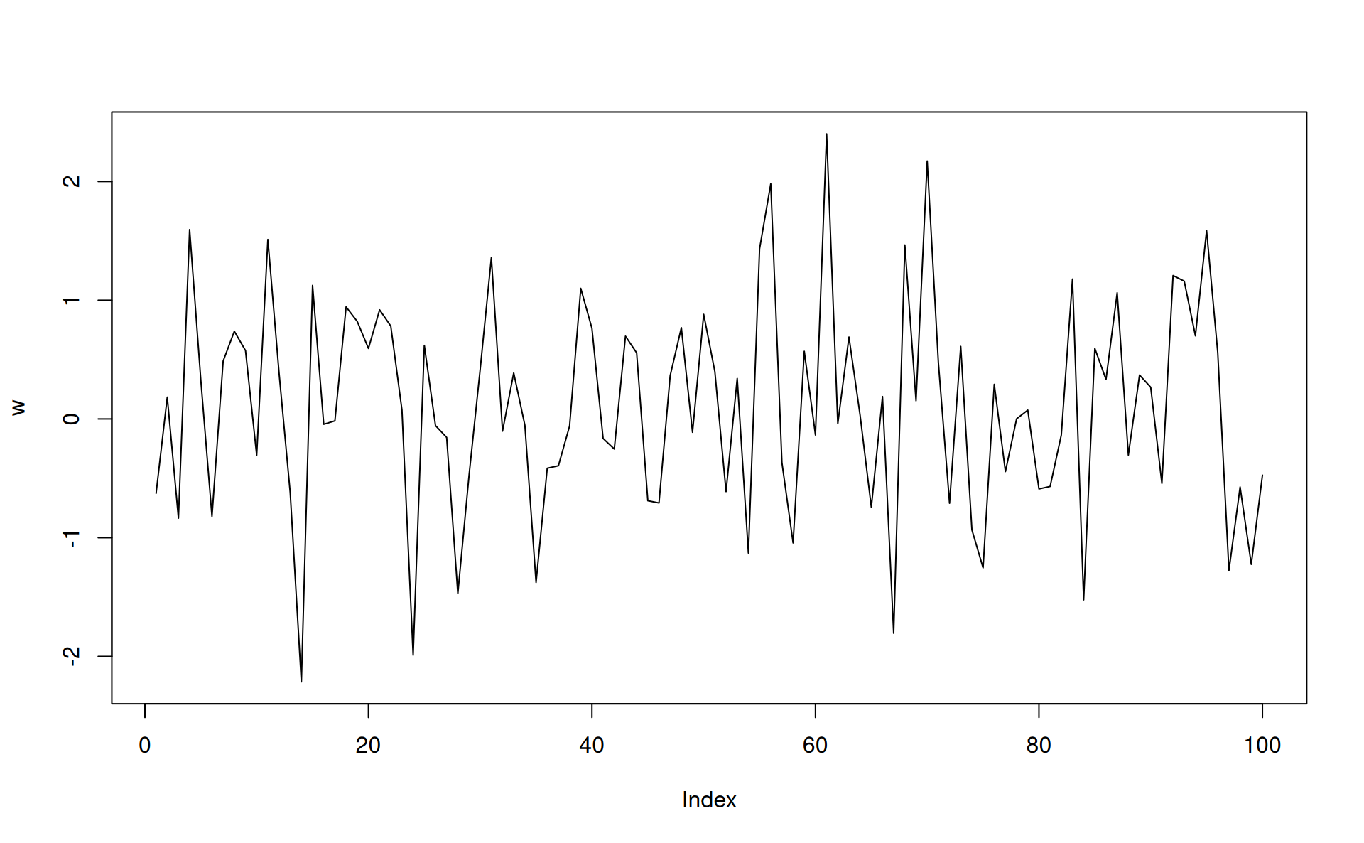
Properties of white noise series
\[\mu_0=0\]
\[\gamma_k=Cov(w_t,w_{t+k})= \begin{cases} \sigma^2 & \text{if} & k=0 \\ 0 & \text{if} & k>0 \end{cases}\]
The autocorrelation function follows as
\[\rho_k = \begin{cases} 1 & \text{if} & k=0 \\ 0 & \text{if} & k \ne 0 \end{cases}\]
Simulated white noise data will not have autocorrelations that are exactly zero (when \(k \ne 0\)) because of sampling variation.
In particular, for a simulated white noise, it is expected that 5% of the autocorrelations will significantly different from zero at 5% significance level
Simulated white noise graph
set.seed(2)
acf(rnorm(100))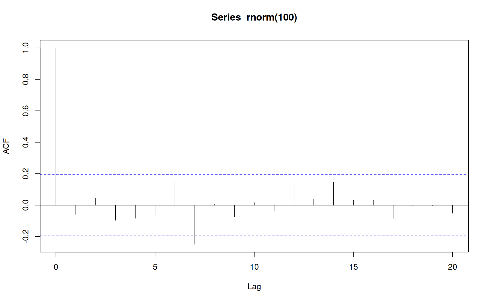 The above is a typical plot, with one statistically significant autocorrelation occurring at lag 7
Fitting a white noise model
A white noise series usually arises as a residual series after fitting an appropriate time series model
The correlogram generally provides sufficient evidence provided the series is of a reasonable length
Only parameter for a white noise series is the variance \(\sigma^2\)
This is estimated by residual variance, adjusted by degree of freedom
4.4 Non-stationary models
4.4.1 Random walks
Introduction
There are mainly two types of trends: deterministic trend and stochastic trend
Series with deterministic trends are relatively easier to handle by detrending or deseasonalizing
On the other hand stochastic trends are those where residuals show deterministic pattern even after detrending and deseasonalizing
A random walk often provides good fit to data with stochastic trends
Though even better fits can be found from more general model formulation, such as ARIMA
Definition of random walk
Let \({x_t}\) be a time series. Then \(x_t\) is a random walk if
\[x_t=x_{t-1}+ w_t\]
where \(\left[w_t\right]\) is a white noise series. Then substituting \(x_{t-1}=x_{t-2}+w_{t-1}\) and then substituting for \(x_{t-2}\) and followed by \(x_{t-3}\) and it gives:
\[x_t= w_t+w_{t-1}+w_{t-2}\]
In practice, the series above will not be infinite but will start at some time \(t=1\),
\[x_t=w_1+w_2+ \ldots + w_t\]
The backward shift operator
The backward shift operator \(B\) is defined by \[Bx_t=x_{t-1}\] The backward shift operator is sometimes called the lag operator. By repeatedly applying B, it follows that \[B^{n}x_t=x_{t-n}\]
Using this backshift operator, we can write
\[x_t=Bx_t+w_t\]