6 General ARMA models

6.1 MA(q) process: Definition and properties

A moving average (MA) process of order \(q\) is a linear combination of the current white noise term

The q most recent past white noise terms and is defined by \[x_t=w_t+\beta_1w_{t-1}+\ldots+\beta_1w_{t-q}\]

Here \({w_t}\) is white noise with zero mean and variance \(\sigma_w^2\).

6.1.1 MA equation with backshift operator

The above equation can be rewritten in terms of the backward shift operator B

\[x_t=(1+\beta_1B+\beta_2B^2+\ldots+\beta_qB^q)wt=\phi_q(B)w_t\]

Here \(\phi_q\) is a polynomial of order \(q\).

MA processes consist of a finite sum stationary white noise terms

They are stationary and hence have a time-invariant mean and autocovariance

6.1.2 Mean and variance of MA process

The mean and variance for \({x_t}\) are easy to derive

The mean is just zero because it is a sum of terms that all have a mean of zero

The variance is \(\sigma{^2}_{w}(1+\beta_1^2+\ldots+\beta^2_q)\)

Each of the white noise terms has the same variance and the terms are mutually independent.

6.1.3 Autocorrelation function and MA process

The autocorrelation function for an \(MA(q)\) process can readily be implemented in R

Note that the function takes the lag \(k\) and the model parameters \(\beta_i\) for \(i=0,1,\ldots,q,\) with \(\beta_0=1\)

6.1.4 R codes

The autocorrelation function is computed in two stages using a for loop

rho <- function(k, beta) {
q <- length(beta) - 1
if (k > q) ACF <- 0 else {
s1 <- 0; s2 <- 0
for (i in 1:(q-k+1)) s1 <- s1 + beta[i] * beta[i+k]
for (i in 1:(q+1)) s2 <- s2 + beta[i]^2
ACF <- s1 / s2}
ACF}

The first loop generates a sum \((s1)\) for the autocovariance

The second loop generates a sum \((s2)\) for the variance with the division of the two sums giving the returned autocorrelation (ACF)

Using the code

Using the code above for the autocorrelation function, correlograms for a range of \(MA(q)\) processes can be plotted against lag

The code in the next slide provides an example for an \(MA(3)\) process with parameters \(\beta_1=0.7, \beta_2=0.5,\) and \(\beta_3=0.2\)

6.1.5 Autocovariance function

beta <- c(1, 0.7, 0.5, 0.2)
rho.k <- rep(1, 10)
for (k in 1:10) rho.k[k] <- rho(k, beta)
plot(0:10, c(1, rho.k), pch = 4, ylab = expression(rho[k]))
abline(0,0)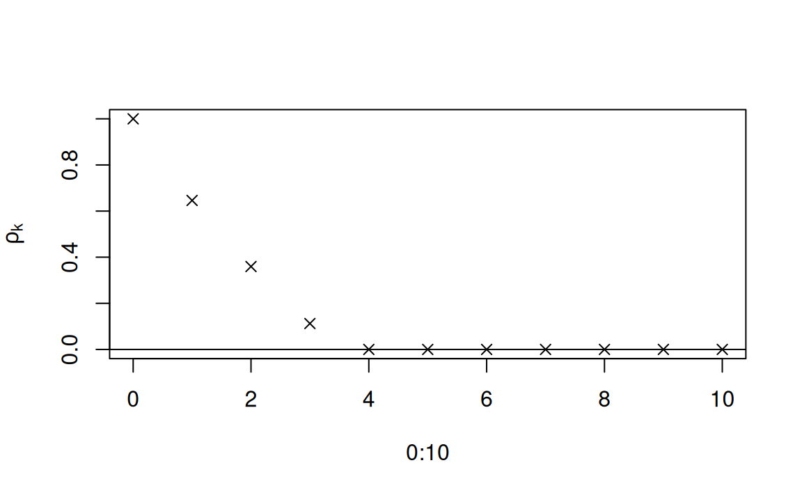

The plot above is the autocovariance function for an \(MA(3)\) process with parameters \(\beta_1=-0.7, \beta_2=0.5, \beta_3=-0.2\)

Negative correlations at lags 1 and 3

The code below can be used to simulate the \(MA(3)\) process

Plot the correlogram of the simulated series

An example time plot and correlogram are show in the figure

As expected, the first three autocorrelations are significantly different from 0

Other statistically significant correlations are attributable ro random sampling variation

In the correlogram plot, 1 in 20 (5%) of the sample correlations for lags greater than 3

Here the underlying population correlation is zero are expected to be statistically significantly different from zero at the 5% level because multiple t-test results are being shown on the plot

set.seed(1)
b <- c(0.8, 0.6, 0.4)
x <- w <- rnorm(1000)
for (t in 4:1000) {
for (j in 1:3) x[t] <- x[t] + b[j] * w[t - j]
}
 plot(x, type = "l")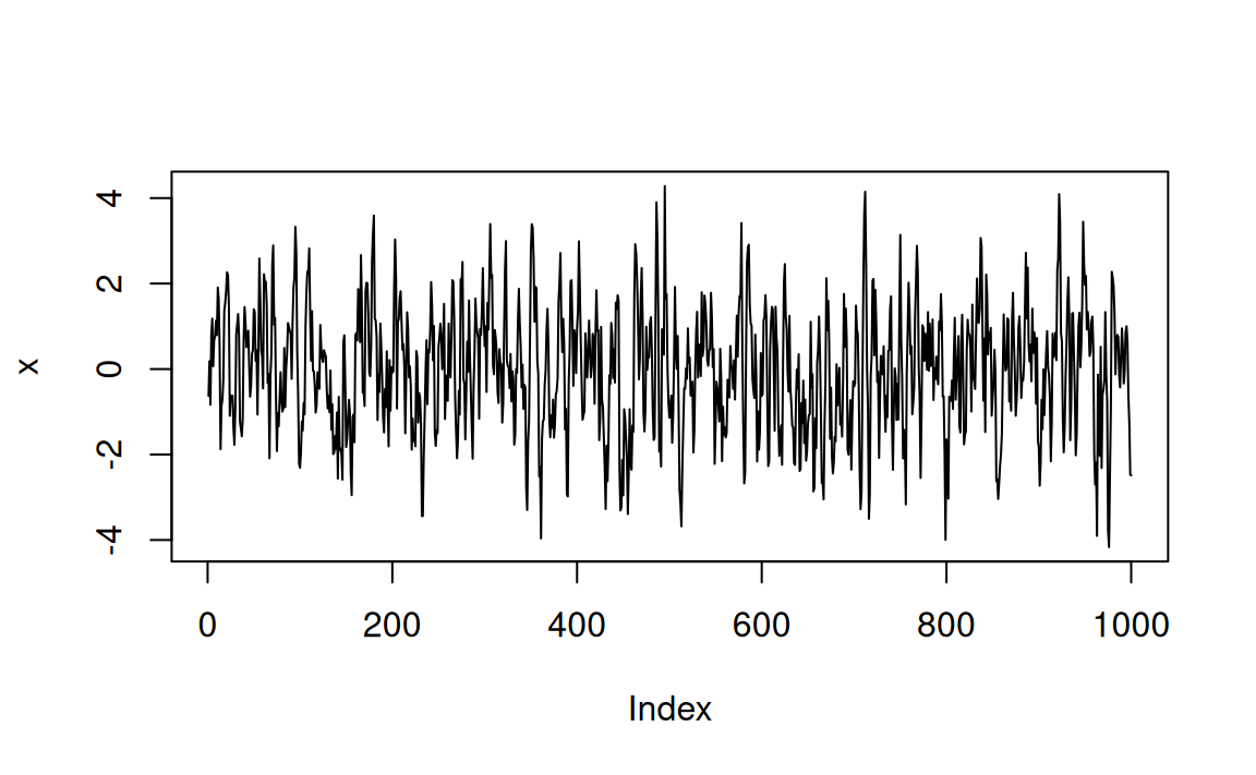

 acf(x)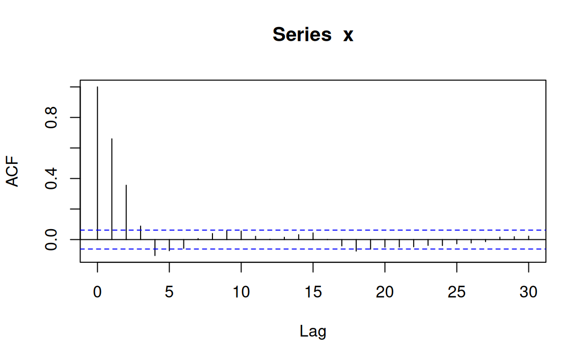

6.1.6 Fitted MA models

Model fitted to simulated series

An \(MA(q)\) model can be fitted to data in R using the arima function with the order function parameter set to c(0,0,q)

Unlike the function ar, the function arima does not subtract the mean by default and estimates an intercept

MA models cannot be expressed in a multiple regression form, the parameters are estimated with a numerical algorithm

The function arima minimises the conditional sum of squares to estimate values of the parameters and will either return these if method=c("CSS") is specified or use them as initial values for MLE

In the following code, a moving average model, x.ma, is fitted to the simulated series of the last section

Looking at the parameter estimates, it can be seen that the 95% confidence interval

approximated by \(coeff.\pm2\) s.e. of \(coeff\)) contain the underlying parameter values (0.8, 0.6 and 0.4) that were used in the simulations.

Furthermore, the intercept is not significantly different from its underlying parameter value of zero

x.ma  <- arima(x, order=c(0,0,3))
x.ma 

Call:
arima(x = x, order = c(0, 0, 3))

Coefficients:
         ma1     ma2     ma3  intercept
      0.7898  0.5665  0.3959    -0.0322
s.e.  0.0307  0.0351  0.0320     0.0898

sigma^2 estimated as 1.068:  log likelihood = -1452.41,  aic = 2914.83

Here is the acf

acf(x.ma$res[-1])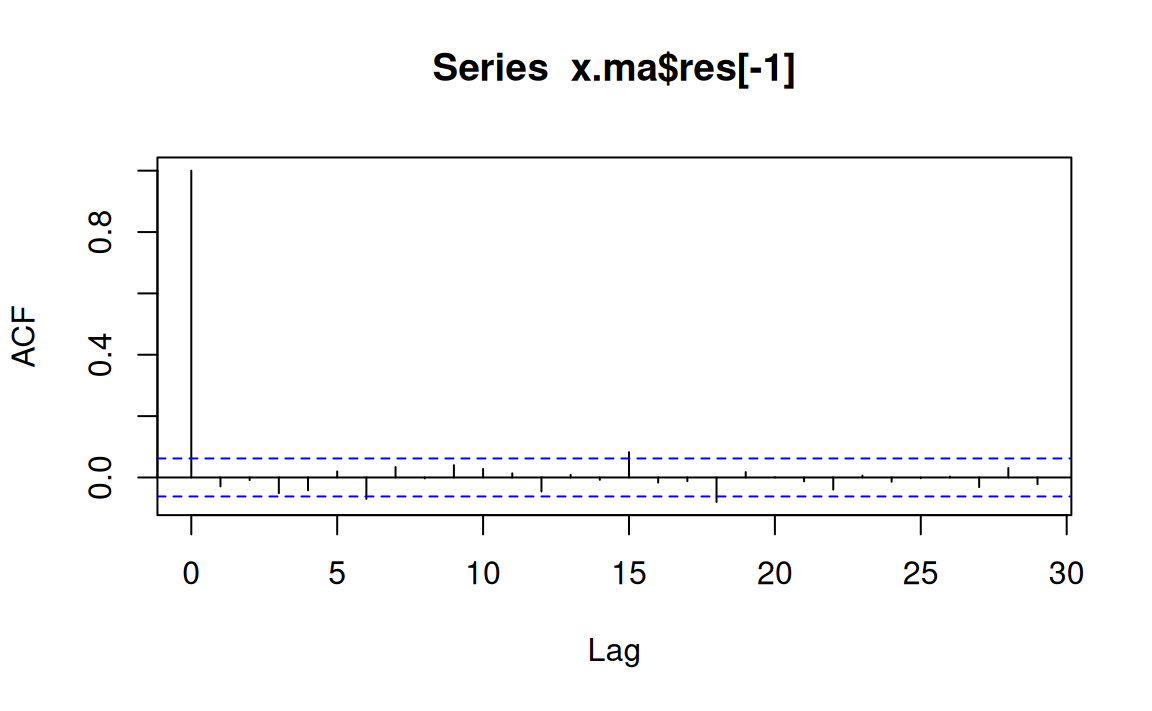

6.1.7 Stationarity

A stochastic process is said to be stationary if it’s properties are unaffected by a change of time origin.Time origin might mean the particular time period which represents the time range. It might be the starting time period or the center value of time. In other words, joint probability distribution of any set of times does not change shape or affected by any means if there is a shift in the time axis. Why we talk about joint probability distribution here. This is because every value in every time period is a particular value of a random variable. For example, \(Y_t\) is random variable, same as \(Y_{t-1}\) is a random variable. When a time-series consists of these two variables, the distribution of this time series is a joint distribution.

Strict stationarity

A time series model \({x_t}\) is strictly stationary if the joint distribution of \(x_1,\ldots,x_{t_n}\) is the same as the joint distribution of \({x_{1+m},\ldots,x_{t+m}}\) for all \(t_1,\ldots,t_n\) and m, so that the distribution is unchanged after an arbitrary time shift.

Strict stationarity implies that the mean and variance are constant in time

Autocovariance \(Cov(x_t, x_s)\) only depends on lag \(k=|t-s|\) and can be written \(\gamma(k)\)

Weak stationarity

If a series is not not strictly stationary but the mean and variance are constant in time and autocovariance only depends on the lag, then the series is called second-order stationary.

Usually stationarity is a very strict condition which requires that the whole distribution must be unchanged at any time period. It means that all the moments in any order should be equal. But this is usually impractical to find. As a result, we impose a softer version of this which we call . Weak stationarity is a situation when we have just mean, variance are equal. We also have covariance which does not change we time difference between variables are the same. This means:

\[\begin{equation} Cov(Y_1,Y_5)=Cov(Y_{17},Y_{21}) \label{eqeqcov} \end{equation}\]

This is also called covariance stationary. We can formally express the covariance stationary in the following way:

\[\begin{align} E(Y_t)&=\mu < \infty \label{eqm}\\ Var(Y_t)&=\sigma^2 \label{eqv}\\ Cov(Y_t,Y_{t-k})&=E[(Y_t-E(Y_{t-1}))(Y_{t-k}-E(Y_{t-k}))] \\ &=E[(Y_t-\mu)(Y_{t-k}-\mu)]\\ &=\gamma_k \label{sco} \quad k=1,2,3,\dotsc \end{align}\]

Here, equation and implies that weakly stationary process is characterized by constant finite mean and variance. On the other hand, implies that covariance between any two time periods does not depend on the time period they are in, rather it depends on the time lag between these two variables.

If the white noise is Gaussian, the stochastic process is commpletely defined by the mean and covariance structure, in the same way as any normal distribution is defined by its mean and variance-covariance matrix.

First step in any should be to check whether there is any evidence of a trend or seasonal effects

If there is we will have to remove them

It is often reasonable to treat the time series of residuals as a realisation of a stationary error series.

Therefore, these models in this topic are often fitted to residual series arising from regression analyses

6.1.8 Autocorreation function (ACF)

Autocovariance

Since here we are trying to find covariance between two variables where one is the lag version of the same variable, we call these . Here we define the as: \[\begin{equation} \gamma_k=Cov(Y_t,Y_{t-k})=Cov(Y_{t-k},Y_t) \label{sco2} \end{equation}\]
When \(k=0\), \(\gamma_k\) reduces to:

\[\begin{equation} \gamma_0=Cov(Y_t,Y_t)=Var(Y_t) \label{gam0} \end{equation}\]

Autocorreation

One problem with covariance its value is not independent of the units in which the variables are measured. For example, \(Cov(Y_1,Y_5)\) and \(Cov(Y_12, Y_16)\) might not equal just because units are different. For example, let’s say \(Y_t\) is measuring the CPI. In early time periods, CPI usually had lower values but suddenly it got a shift in later time periods. It’s better to use correlation measure which is unit free, obviously we will use which standardizes to compare across different series. Here we will derive \(\rho_k\) which is the k-th order autocorreation:

\[\begin{align} \rho_k & =\frac{Cov(Y_t,Y_{t-k})}{\sqrt{Var(Y_t)}\sqrt{Var(Y_{t-1})}} \\ & =\frac{\gamma_k}{\gamma_0} \quad (\text{by}\quad \eqref{gam0}) \label{eqrho} \end{align}\]

Obviously, here \(\rho_0=\frac{Cov(Y_t,Y_t)}{\gamma_0}=\frac{Var(Y_t)}{\gamma_0}=\frac{\gamma_0}{\gamma_0}=1\). And also as usual, $-1_k $ which is standard for autocorrelation measures.

Autocorrelation Function(ACF)

Autocorrelations as a function of lag order \((k)\) is called autocorrelation function or ACF. ACF plays a major role in understanding a time series. It tells us how deep is the memory of the underlying stochastic process. If it has long memory, as in the case of \(AR(1)\), we would see that value of \(\rho_k\) does not diminish to zero with increasing value of \(k\) as quickly as the \(MA(1)\) does.We already have seen that in section that covariance between two periods, in a \(MA(1)\) process, reduces to zero if lag is just more than one period. Therefore by looking into the ACF we can have a fair idea about the underlying time series stochastic process.

ACF of \(AR(1)\) and \(MA(1)\)

We have just previously seen that we can express autocorrelation of order \(k\) as : \[\begin{equation} \rho_k=\frac{\gamma_k}{\gamma_0} \label{} \end{equation}\] In the case of \(AR(1)\), we have seen that in one of the previous equations that: \[\begin{align} Cov(Y_t,Y_{t-k}) & =\rho_k \\ & =\theta^k \frac{\sigma^2}{1-\theta^2} \\ &=\theta^k \gamma_0 \\ \text{And, we also have seen that} Var(Y_t) & =\gamma_0=\frac{\sigma^2}{1-\theta^2}\\ \text{So, we can say that, in the case of $AR(1)$} \rho_k & =\frac{\gamma_k}{\gamma_0} \\ &=\theta^k \frac{\cancel{\gamma_0}}{\cancel{\gamma_0}} &=\theta^k \label{} \end{align}\]

Ikn the case of \(MA(1)\), we also have seen previously that : \[\begin{align} \gamma_1 & =Cov(Y_t,Y_{t-1})=\alpha \sigma^2,\quad \text{and}\\ \gamma_0 & =Var(Y_t)= \sigma^2 (1+\alpha^2) \\ \text{Therefore, from the above two we can write} \rho_1 & =\frac{\gamma_1}{\gamma_0} \\ &=\frac{\alpha \cancel{\sigma^2}}{\cancel{\sigma^2}(1+\alpha^2)} &=\frac{\alpha}{1+\alpha^2} \label{} \end{align}\]

And in the case of $k $, we have also seen that \(\gamma_k=0 \quad \forall k\). Therefore,

\[\begin{equation} \rho_k=0 \quad \forall \quad k \label{} \end{equation}\]

Implication of the above derivation is that, a shock in \(MA(1)\) will only last two period, \(Y_t\) and \(Y_{t-1}\) while a shock in \(AR(1)\) will affect all future observations with a decreasing effect, since \(|\theta|<1\).

Graphical Representation

Graphs of simulatated \(AR(1)\) and \(MA(1)\) goes in here.

6.2 Formulating ARMA process

In this section, we start to define more general autoregressive and moving average process. First we define a moving average of order q: \[\begin{equation} y_t=\varepsilon_t+\alpha_1 \varepsilon_{t-1}+\alpha_2 \varepsilon_{t-2}+\dotsb+\alpha_q \varepsilon_{t-q} \label{eq:maq} \end{equation}\] Here, \(y_t=Y_t-\mu\) and \(\varepsilon_t\) is a white noise process. It also means that the demeaned series \(y_t\) is a weighted combination (can we say weighted average also?) of \(q+1\) white noise terms. Here is \(q+1\) terms since the \(q\) starts from the second term. On the other hand, an autoregressive process of order \(p\), which is denoted as \(AR(p)\), can be expressed as:

\[\begin{equation} y_t=\theta_1 y_{t-1}+\theta_2 y_{t-2}+\theta_3 y_{t-3}+\dotsb+\theta_p y_{t-p}+\varepsilon_t \label{eq:arq} \end{equation}\]

Obviously it is very much possible to combine the \(MA(q)\) and \(AR(p)\) and come up with a \(ARMA(p,q)\) specification of the following form: \[\begin{equation} y_t=\theta_1 y_{t-1}+\theta_2 y_{t-2}+\dotsb+\theta_p y_{t-p}+\varepsilon_t+\alpha \varepsilon_{t-1}+\dotsb+\alpha_q \varepsilon_{t-q} \end{equation}\] Now, the next million dollar question is when to choose an \(AR\), \(MA\) or \(ARMA\)? Verbeek remains quite vague about this at this point. He says, \(AR\) and \(MA\) basically same time of series. It’s just a matter of parsimony. What’s the meaning of this? We have previously seen that \(AR(1)\) can be expressed as infinte lag order of \(MA\) series. So, what does parsimony means here? Does this mean that if we weant a smaller model then we choose \(AR(1)\) over infinite order \(MA\)? Verbeek says it will be clear later. At this point, it is difficult to know. We will postpone the discussion for now, come back to it later. Now we will talk briefly on .

6.2.1 Lag operator

In the notation of time series model, it is often convenient to use lag operator(\(L\)) or backshift operator(\(B\)) which some author use. But we will stick to \(L\) here. Let’s see a use: \[\begin{equation} Ly_t=y_{t-1}\\ L^2y_t=L.Ly_t=L.y_{t-1}=y_{t-2}\\ \vdots \\ L^q y_t=y_{t-q} \label{} \end{equation}\]
There are other relationships involving \(L\), such as \(L^0 \equiv 1\) and \(L^{-1}=y_{t+1}\). Use of this notions makes life much simpler in specifying a long time series specification such as an \(ARMA\) model quite concisely. For example, let’s start with an \(AR(1)\) model:

\[\begin{equation} \begin{split} y_t & =\theta y_{t-1}+\varepsilon_t \\ & =\theta L.y_t+\varepsilon_t \\ y_t-\theta Ly_t & = \varepsilon_t \\ (1-\theta L)y_t &= \varepsilon_t \end{split} \label{eq:eqL} \end{equation}\]

We can refer to as follows: here, \(y_t\) and it’s one period lag \(y_{t-1}\) , on the right hand side, is a combination with weights of 1 and \(-\theta(L)\) and equals a white noise process (\(\varepsilon_t\)). In general, we can write \(AR(p)\) as follows: \[\begin{equation} \theta(L)y_t=\varepsilon_t \label{eq:eqargen} \end{equation}\] Here \(\theta(L)\) is a polynomial of order \(p\) . I think \(\theta(L)\) is some kind of function of \(L\). We could write it like \(f(L)\). Writing it like \(\theta(L)\) creates some confusion because there is also \(\theta\) in the function. Now, \(\theta(L)\) can be expressed as: \[\begin{equation} \theta(L)=1-\theta L -\theta_2 L^2-\dotsb-\theta_p L^p \label{eqlagpol} \end{equation}\] We can interpret lag polynomial as a filter. When we apply it to a time series, it produces a new series.

6.2.2 Characteristics of Lag Polynomial

Suppose we apply a lag polynomial to a time series. Then we apply another lag polynomial on the top of that series. This is equivalent to applying product of two lag polynomial on the original series. We can also define the inverse of a filter, which is the inverse of polynomial. The inverse of \(\theta(L)\) is \(\theta^{-1}(L)\) and we can write \(\theta(L) \theta^{-1}(L)=1\) . Now the following statement I really don’t understand.

If \(\theta(L)\) is a finite order polynomial, then \(\theta{-1}L\) is a infinite order polynomial in \(L\). It also goes onto claim that \[\begin{equation} (1-\theta L)^{-1}=\sum_{j=0}^{\infty}\theta^j L^j \label{eq:lagpol2} \end{equation}\]

provided that \(|\theta|<1\). Now the question is how to prove that claim? Now let’s start with simply \(\sum_{j=0}^\infty \theta^j\).

\[\begin{align} \sum_{j=0}^\infty & = \theta_0+\theta_1+\dotsb \\ & =\frac{1-\theta^\infty}{1-\theta} \quad \text{provided that} \quad |\theta|<1 \\ &=\frac{1}{1-\theta} \label{eq:eqthet} \end{align}\] Now let’s see this version: \[\begin{align} \sum_{j=0}^\infty \theta^j L^j & = \theta^0 L^0+ \theta^1 L^1 + \theta^2 L^2+ \dotsb \\ & = 1+\theta L + \theta^2 L^2+\dotsb \\ & = \frac{1-(\theta L)^\infty}{1-\theta L} \\ & = \frac{1-\theta^\infty L^\infty}{1-\theta L} \\ & = \frac{1}{1-\theta L} \quad \text{by} \quad |\theta|<1\\ & = (1-\theta L)^{-1} \\ \text{So we find that,} \sum_{j=0}^\infty \theta^j L^j & = \frac{1}{1-\theta L}=(1-\theta L)^{-1} \label{eqthl} \end{align}\]

Now, we have seen in that \((1-\theta L)y_t=\varepsilon_t\). From this it follows that: \[\begin{align} (1-\theta L)^{-1}(1-\theta L) y_t & = (1-\theta L)^{-1} \varepsilon_t \\ y_t & = (1-\theta L)^{-1} \varepsilon_t \\ \text{or,} \qquad y_t & = \sum_{j=0}^\infty \theta^j L^j \varepsilon_t \\ \text{From, the previous definition of Lag operator($L$)} L\varepsilon_t & = \varepsilon_{t-1} \\ L^2 \varepsilon_t & =\varepsilon_{t-2} \\ \vdots \\ L^j \varepsilon_t &= \varepsilon_{t-j} \\ \text{Therefore, we can write} y_t & = \sum_{j=0}^\infty \theta^j \varepsilon_{t-j} \label{} \end{align}\]

6.3 From \(MA(1)\) to AR(\(\infty\))}

It corresponds to same derivation where we have shown that \(AR(1)\) corresponds to \(MA(\infty)\) series. We have said previously that \(MA(1)\) can also be transformed into a \(AR\) series but could not show it quite mathematically. Armed with lag operator \((L)\), we can try to show it here. \[\begin{align} \text{We know that in $MA(1)$} y_t &= \varepsilon_t+\alpha \varepsilon_{t-1} \\ &= \varepsilon_t+\alpha L \varepsilon_t \\ &= (1+\alpha L)\varepsilon_t (1+\alpha L)^{-1}y_t &= \varepsilon_t \end{align}\]

Now, let’s see how we can define \((1+\alpha L)^{-1}\).

\[\begin{align} (1+\alpha L)^{-1} &= \frac{1}{(1+\alpha L)} \\ & = \frac{1-(-\alpha L)^{\infty}}{1-(-\alpha L)} \\ & = -\alpha L+(-\alpha L)^2+ (-\alpha L)^3+\dotsb \\ & = \sum_{j=0}^\infty (-\alpha L)^j \\ \text{Therfore, we write that } (1+\alpha L)^{-1} & = \sum_{j=0}^\infty (-\alpha L)^j \\ \text{Basically, we see that} \varepsilon_t &=\sum_{j=0}^\infty (-\alpha)^j (L)^j y_t\\ &=\sum_{j=0}^\infty (-\alpha)^j y_{t-j} \text{Now, let's figure out $\varepsilon_{t-1}$. This is important since we write $MA(1) = \alpha \varepsilon_{t-1}+\varepsilon_t$. What we will do is put the value of $\varepsilon_{t-1}$ and keep $\varepsilon_t$ as it is} y_{t-1} & =\varepsilon_{t-1}+\alpha \varepsilon_{t-2} \\ & =\varepsilon_{t-1} + \alpha L \varepsilon_{t-1} \\ & =\varepsilon_{t-1}(1+\alpha L) \\ \text{or,}\qquad \varepsilon_{t-1} & =(1+\alpha L)^{-1} y_{t-1} \\ & = \sum_{j=0}^\infty (-\alpha L)^j y_{t-1} \\ & = \sum_{j=0}^\infty (-\alpha)^j L^j y_{t-1} \\ & = \sum_{j=0}^\infty (-\alpha)^j y_{t-j-1} \\ \text{So, we can write} \varepsilon_{t-1} &= \sum_{j=0}^\infty (-\alpha)^j y_{t-j-1} \\ \text{Now getting back to the $MA(1)$,} y_t & =\alpha \varepsilon_{t-1}+\varepsilon_t \\ & =\alpha \sum_{j=0}^\infty (-\alpha)^j y_{t-j-1}+ \varepsilon_t \\ \end{align}\]

We here require that in the \(MA(1)\) which is \((1+\alpha L)\) is invertible. It can be shown that it is invertible only if \(|\alpha|<1\). \(AR\) representation is very convenient when we think that current behavior is determined by past behavior. \(MA\) representation is quite useful for determining variance and covariance of the process. It is not quite clear how so but it might be clear in the subsequent analysis.

6.4 Parsimonious representation of ARMA

We have seen previously the following \(ARMA\) representation: \[\begin{gather} y_t =\theta_1 y_{t-1}+\theta_2 y_{t-2}+\dotsb+\theta_p+\varepsilon_t+\alpha \varepsilon_{t-1}+\dotsb+\alpha_q \varepsilon_{t-q} \\ \text{or,} \qquad y_t-\theta_1 y_{t-1}-\dotsb-\theta_p y_{t-p} =(\alpha(L))\varepsilon \\ \text{or,} \qquad \theta (L) y_t =\alpha (L) \varepsilon_t \\ \text{Now, if we think lag polynomical in $AR(1)$ is invertible, then} y_t =\theta^{-1}(L) \alpha (L) \varepsilon_t \\ \text{On the other hand, if lag polynomial in $MA(1)$ is invertible, then we can write} \alpha^{-1}(L) \theta (L) y_t =\varepsilon_t \label{eq:eqpararma} \end{gather}\]

6.5 Invertibility of Lag Polynomial

6.5.0.1 Generalization

We have seen that for the first order lag polynomical \(1-\theta L\) is invertible if \(|\theta|<1\). But it is not clear at this point what we mean by invertibility. Is this means whether we can find the value of \(\frac{1}{1-\theta L}\)? We can find the value of this expression even though \(|\theta|>1\), it’s just negative. Now, whatever invertibility is, let’s move onand try to generalize this condition. First start with a second order polynomial. Then we will move onto higher degree of polynomial.

6.5.1 Second Order Polynomial

Let’s consider this second order polynomial:

\[\begin{equation} 1-\theta_1 L-\theta_2 L^2 \label{eq:eq2pn} \end{equation}\] How to solve this type of question? Well this is typically a equation of the following form: \[\begin{equation} \label{eq2gn} ax^2+bx+c \end{equation}\] Here \(a=-\theta_2, b=-\theta_1, c=1\). Now the typical solution for this type of equation is: \[\begin{align} x & =\frac{-b\pm \sqrt{b^2-4ac}}{2a} \label{eq:eqax2} \end{align}\]

Now let's think about a numerical example with the following example:  

\[\begin{multline}\label{eqnumex} x^2-8x+15=x^2-3x-5x+15=x(x-3)-5(x-3) \\ =(x-3)(x-5)=(3-x)(5-x)=15(1-x/3)(1-x/5) \end{multline}\]

Now let’s put the above numerical example into a general mathematical form:

\[\begin{equation}\label{eqphi} 1-\theta_1 L-\theta_2 L^2=(1-\varphi_1 L)(1-\varphi_2 L) \end{equation}\]

Now if we look into and compare it with , we find that \(\varphi_1=1/3\) and \(\varphi_2=1/5\). But the presence of \(15\) complicates the matter. Anyway, let’s whether we can resolve the issue or not. Author says that we can write \(\varphi_1+\varphi_2=\theta_1\).It sounds like for the usual quadratic equation formula in there is some relation.

Now look into to relate itto the numerical example we have. If we think \(\varphi_1=1/3\) and \(\varphi_2=1/5\), then \(\varphi_1+\varphi_2=1/3+1/5=\frac{5+3}{15}=8/15\). Now we see what complicates the situation, its the \(15\). If we compare and , then we can say that \(\theta_1=8\). Then \(\varphi_1+\varphi_2=8/15\) does not quite equal to \(15\). But if we multiply it by \(15\) then \(\frac{\cancel{15}}{8/\cancel{15}}=8\).

The relationship is also such that \(-\varphi_1 \varphi_2= \theta_2\). Now let’s check whether this holds. We have \(1/3 \cdot 1/5=1/15\). But again we have to multiply by \(15\) to get the desired result. Hence we get \(1\) which is equivalent to \(\theta_2=1\) which is the coefficient of \(x^2\) in .Ok that is fine.

6.5.1.1 Condition for invertibility

But the part that I don’t understand is the condition for invertibility in the polynomial. It says that the polynomial of second order in will be invertible if both of the first order polynomials are also invertible. The first order polynomials are: \((1-\varphi_1 L)\) and \((1-\varphi_2 L)\) . These two have to be also invertible for the whole quadratic polynomial to be invertible . This implies that both \(\varphi_1\) and \(\varphi_2\) has to be less than one, that is : \[\begin{equation} |\varphi_1| < 1 \qquad \text{and} |\varphi_2| < 1 \label{eqphi2} \end{equation}\]

Why this is so is not clear. Have to look into greater details. Anyways, author moves on to say that these requirements can also be formulated in terms of the so-called . Does it mean that charateristic equation is another way to mention this requirements of invertibility? Anyway, let’s first specify the characteristic equation: \[\begin{equation} (1-\varphi_1 z)(1-\varphi_2 z)=0 \label{eqphi3} \end{equation}\] When we look into this equation, the first thing that comes to mind is that why we are suddenly using \(z\) instead of \(L\) as we have done in .Well, my guess is that, it has been probably done to give a more generic look of the chracteristic equation. That’s the only explanation I can find here.

Solution of the equation in can be expressed by two values of \(z\): \(z_1\) and \(z_2\). These are called .Why this is called characteristic equation or characteristic roots? Now the invertibility condition requires that \(|\varphi_i|<1\) which translates into \(|z_i>1|\). If any solution that satisfies \(|z_i|\ge 1\) will result into a non-invertible polynomial. If \(|z_i|\) is exactly equal to \(1\), then that solution is referred to as .

Invertibility with lag polynomial coefficients Here the author discusses an easier to detect the presence of unit root in a lag polynonmial. Remember, here we are talking about lag polynomial not the equation itself. It may create some confusion in the beginning. It certainly did in my case. Now the statement that confused me is the following:

We can detect the presence of unit root by noting that the polynomial \(\theta(z)\) evaluated at \(z=1\) is zero if \(\sum_{j=1}^{p} \theta_j=1\). Thus the presence of a first unit root can be verified by checking whether the sum of polynomial coefficients equals one. If the sum exceeds one, the polynomial is not invertible.

Now have a look at the above statement and try to evaluate it with the following example. We are considering the following \(AR(2)\) model:

\[\begin{equation}\label{eqexm} y_t=1.2 y_{t-1} - 0.32 y_{t-2}+\varepsilon_t \end{equation}\]

Now having a look at this equation , we might think that \(\sum_{j=1}^{2}=1.2+(-0.32)=0.70\) which is less than one. This might work just fine. We can express this equation a little bit more elaborately in the lag polynomial form:

\[\begin{gather}\label{eqexm2} y_t =1.2 L y_t-0.32 L^2 y_t+\varepsilon_t \\ y_t(1-1.2L+0.32 L^2)=\varepsilon_t \text{We can also write this as} y_t(1-0.8L-0.4L+0.32L^2)=\varepsilon_t \\ y_t[(1-0.8L)-0.4L(1-0.8L)]=\varepsilon_t \\ y_t(1-0.8L)(1-0.4L)=\varepsilon_t \text{This corresponds to the characteristics equation of the following form:} 1-1.2z+0.32z^2=(1-0.4z)(1-0.8z)=0 \end{gather}\]

Now let’s revisit the following statement and try to relate it with the above statement: We can detect the presence of unit root by noting that the polynomial \(\theta(z)\) evaluated at \(z=1\) is zero if \(\sum_{j=1}^{p} \theta_j=1\). Thus the presence of a first unit root can be verified by checking whether the sum of polynomial coefficients equals one. If the sum exceeds one, the polynomial is not invertible.

Now let’s check what would be the value of characteristics equation when evaluated at \(z=1\).

\[\begin{gather} 1-1.2z+0.32z^2=1-1.2(1)+0.32(1)^2=1-1.2+0.32=1-0.70=0.30 \end{gather}\]

We find the value of characteristics equation becomes \(0.30\) when z=1. When this value will become \(0\)? Now to see that let’s consider the equation when this value might become zero. How about this equation:

\[\begin{equation}\label{eqexmv2} y_t=1.2y_{t-1}-0.2y_{t-2}+\varepsilon_t \end{equation}\]

Here some of the coefficeints in the lag polynomial will be \(1.2-0.2=1\). Now what is wrong with that? Now the left hand side of the chracteristics equation with \(z=1\) will be: \[1-1.2z+0.2z=1-1.2+0.2=0\] Here we see that when sum of the coefficients of the polynomial is \(1\), then value of the polynomial is zero when \(z=1\).

Consequences of Invertibility Now what’s the consequence of this? It’s still not clear to me. In this case of a simple example it is obvious. For example: \[\begin{equation}\label{eqrw} y_t=1.2y_{t-1} +\varepsilon_t \end{equation}\]

Here, lag polynomial is much simpler: \(1-1.2L\). Sum of the lag polynomial here is \(1.2\) where there is only first degree lag, so we have just one term here. It is greater than \(1\), so it must be invertible. The real signficance of invertibility is that the series becomes non-stationary. At least that what I understood. The border line case is the value of lag coefficient is 1.

\[ y_t=y_{t-1}+\varepsilon_t \]

The issue of whether lag polynomials are invertible or not is important for serveral reasons.For moving average models, it is important for estimation and predictions. For the autoregressive models, we already mentioned, it’s ensures stationarity.

Common Roots Now here we will talk about common roots. Let’s have a look into the \(ARMA(2,1)\) process of the following form: \[\begin{gather} \label{} y_t=\theta_1 y_{t-1}+\theta_2 y_{t-2}+ \varepsilon_t + \alpha_1 \varepsilon_{t-1} \\ y_t=\theta_1 L.y_t+\theta_2 L^2 y_t+\varepsilon_t+\alpha_1 L.\varepsilon_t \\ y_t[1-\theta_1 L -\theta_2 L^2]=\varepsilon_t[1+\alpha_1 L]\\ y_t(1-\varphi_1L)(1-\varphi_2 L)=\varepsilon_t(1+\alpha_1 L)\\ \text{Now, if $\alpha_1=-\varphi_1$} y_t(1+\alpha_1 L)(1-\varphi_2 L)=\varepsilon_t(1+\alpha_1 L)\\ y_t \cancel{(1+\alpha_1 L)}(1-\varphi_2 L)=\varepsilon_t\cancel{(1+\alpha_1 L)} y_t(1-\varphi_2 L)=\varepsilon_t \end{gather}\]

In the above we see that we start with a process \(ARMA(2,1)\) and end up with a \(ARMA(2-1,1-1)\) or \(AR(1)\) process. Because fo the cancelling root, it seem they are equivalent which is wrong. In general. becasue of one canceling root \(ARMA(p,q)\) can be written as \(ARMA(p-1, q-1)\).

An example can better illustrate the situation but above explantion might suffice here. The issue is that with a common cancelling root it is difficult to identify which one is the real underlying stochastic process.

A time series will often have well-defined components: trend and seasonal patterns

A well chosen linear regression may account for these non-stationary components

In this case the residuals from the fitted model should not contain noticeable trend or seasonal patterns

But unfortunately that does not happen always

Residuals will usually be correlated in time, this is not accounted for in the fitted regression model

This happens because similar values may cluster together in time

Adjacent observations may be negatively correlated, for example high monthly sales figure may be followed by an unusually low value because customers have supplies left over from the previous month

In this topic, we consider stationary models that may be suitable for residual series that contain no obvious trends of seasonal cycles

The fitted stationary models may then be combined with the fitted regression model to improve forecasts

The autoregressive models that were introduced often provide satisfactory models for the residual time series.

6.6 Mixed models: The ARMA process

Definition

An AR(p) process can be described in the following manner:

\[x_t=\alpha_1x_{t-1}+\alpha_2x_{t-2}+\ldots+\alpha_px_{t-p}+w_t\]

Here \({w_t}\) is white noise and the \(\alpha_i\) are the model parameters.

A useful class of models are obtained when AR and MA terms are added together in a single expression

A time series \({x_t}\) follows an autoregressive moving average (ARMA) process of order \((p,q)\), denoted \(ARMA(p,q)\) when

\[x_t=\alpha_1x_{t-1}+\alpha_2x_{t-2}+\ldots+\alpha_px_{t-p}+w_t+ \beta_1w_{t-1)+\beta_2w_{t-2}+\ldots+\beta_qw_{t-q}\]

Here \({w_t}\) is white noise

The above equation can be represented in terms of the backward shift operator B and rearranged in the more concise polynomial form

\[\theta_p(B)x_t=\phi_q(B)w_t\]

The following points should be noted about an ARMA(p,q) process:

The process is stationary when the roots of \(\theta\) all exceed unity in absolute value

The process is invertible when the roots of \(\phi\) all exceed unity in absolute value

The AR(p) model is the special case \(ARMA(p,0)\)

The MA(q) model is the special case ARMA(0,q)

Parameter parsimony : When fitting to data, an ARMA model will often be more parameter efficient - require fewer parameters - than a single MA or AR model

Parameter redundancy: when \(\theta\) and \(\phi\) share a common factor, a stationary model can be simplified. For example, the model \((1-\frac{1}{2}B)(1-\frac{1}{3})x_t=(1-\frac{1}{2})w_t\)$ can be written as \((1-\frac{1}{3})x_t=wt\)

ARMA models: Empirical analysis

Simulation and fitting

The ARMA process can be simulated using the R function arima.sim

This function takes a list of coefficients representing the AR and MA parameters.

An ARMA(p,q) model can be fitted using the arima function with the order function parameter set to c(p,0,q)

The fitting algorithm proceeds similarly to that for a MA process.

The fitting algorithm proceeds similarly to that for an MA process

Below data from an ARMA(1,1) process are simulated for \(\alpha\)=-0.6 and \(\beta\)=0.5

As expected, the sample estimates of \(\alpha\) and \(\beta\) are close to the underlying model parameters

set.seed(1)
x <- arima.sim(n = 10000, list(ar = -0.6, ma = 0.5))
coef(arima(x, order = c(1, 0, 1)))

         ar1          ma1    intercept 
-0.596966371  0.502703368 -0.006571345 

Exchange rate series

Previously, we have found that a simple MA(1) model failed to provide an adequate fit to the exchange rate series.

In the code below, fitted MA(1), AR(1) and ARMA(1,1) models are compared using the AIC

ARMA(1,1) model provides the best fit to the data, followed by AR(1) model, along with MA(1) model providing the poorest fit.

The figure indicates that the residuals of the fitted ARMA(1,1) model have small autocorrelations

This is consistent with a realisation of white noise and supports the use of the model

x.ma <- arima(x.ts, order = c(0, 0, 1))
x.ar <- arima(x.ts, order = c(1, 0, 0))
x.arma <- arima(x.ts, order = c(1, 0, 1))

Now let’s find the AIC’s

AIC(x.ma)
AIC(x.ar)
AIC(x.arma) 
acf(resid(x.arma))

Electricity production series

Let’s consider the Australian electricity production series

The data exhibit a clear positive trend and a regular seasonal cycle

The variance increases with time

This suggests a log-transformation may be appropriate

A regression model is fitted to the logarithms of the original series in the code below

www <- "http://www.massey.ac.nz/~pscowper/ts/cbe.dat"
CBE <- read.table(www, header = T)
Elec.ts <- ts(CBE[, 3], start = 1958, freq = 12)
Time <- 1:length(Elec.ts)
Imth <- cycle(Elec.ts)
Elec.lm <- lm(log(Elec.ts) ~ Time + I(Time^2) + factor(Imth))
acf(resid(Elec.lm))

The correlogram of the residuals appears to cycle with a period of 12 months suggesting that the monthly indicator variables are not sufficient to account for the seasonality in the series

When we study ARIMA, we will find that this can be accounted for using a non-stationary model with a stochastic seasonal component.

In the meantime, the best fitting \(ARMA(p,q)\) model can be chosen using the smallest AIC either by trying a range of combinations of \(p\) and \(q\) in the arima function

Or using a for loop with upper bounds on \(p\) and \(q\)

In each step of the for loop, the AIC of the fitted model is commpared with the currently stored smallest value

If the model is found to be an improvement, that is it has smaller AIC value, then the new value and model are stored

To start with, best.aic is initialised to infinity \(Inf\)

After the loop is complete, the best model can be found in best.order

In this case, the best model turns out to be an AR(2) model

best.order <- c(0, 0, 0)
 best.aic <- Inf
 for (i in 0:2) for (j in 0:2) {
fit.aic <- AIC(arima(resid(Elec.lm), order = c(i, 0,
j)))
if (fit.aic < best.aic) {
best.order <- c(i, 0, j)
best.arma <- arima(resid(Elec.lm), order = best.order)
best.aic <- fit.aic
}}

Now let’s see the best order

best.order 

Now time for the ACF

acf(resid(best.arma))

The predict function can be used to both to forecast future values from the fitted regression model

Forecast the future errors associated with the regression model suing the ARMA model fitted to the residuals from the regression

These two forecasts can then be summed to give a forecasted value of the logarithm for electricity production

This would need to be anti-logged and perhaps adjusted using a bias correction factor

predict is a generic R function, it works in different ways for different input objects and classes

For a fitted regression model of class lm, the predict function requires the new set of data to be in the form of a data frame

For a fitted ARMA model of class arima, the predict function requires just the number of time steps ahead for the desired forecast

In the latter case, predict produces an object that has both the predicted values and their standard errors

These two values can be extracted using pred and se

In the code below, the electricity production for each month of the next three years is predicted

 new.time <- seq(length(Elec.ts), length = 36)
 new.data <- data.frame(Time = new.time, Imth = rep(1:12,
3))
 predict.lm <- predict(Elec.lm, new.data)
 predict.arma <- predict(best.arma, n.ahead = 36)
 elec.pred <- ts(exp(predict.lm + predict.arma$pred), start = 1991,
freq = 12)
 ts.plot(cbind(Elec.ts, elec.pred), lty = 1:2)

The plot of the forecasted values suggests that the predicted values for winter may be underestimated by the fitted model

This may be due to the remaining seasonal autocorrelation in the residuals

This problem will be tackled in ARIMA topic

Wave tank data

The data in the file wave.dat are the surface height of water (mm), relative to the still water level

This is measured using a capcitance probe positioned at the centre of a wave tank

The continuous voltage signal from this capacitance probe was sampled every 0.1 second over a 39.6 second period.

The objective is to fit a suitable ARMA(p,q) model that can be used to generate a realsistic wave input to a mathematical model for an ocean-going tugboat in a computer simulation

The results of the computer simulation will be compared with tests using a physical model of the tugboat in the wave tank

The pacf suggest that \(p\) should be at least 2

The best fitting ARMA(p,q) model based on a minimum variance of residuals was obtained with both \(p\) and \(q\) equal to 4. The acf and pacf of the residuals from this model are consistent with the residuals being a realisation of white noise.

www <- "http://www.massey.ac.nz/~pscowper/ts/wave.dat"
wave.dat <- read.table(www, header = T)
attach (wave.dat)
layout(1:3)
plot (as.ts(waveht), ylab = 'Wave height')
acf (waveht)
pacf (waveht)
wave.arma <- arima(waveht, order = c(4,0,4))
acf (wave.arma$res[-(1:4)])
pacf (wave.arma$res[-(1:4)])
hist(wave.arma$res[-(1:4)], xlab='height / mm', main='')