Chapter 3 Methods

3.1 Dealing with Corrupted Data

To reintroduce the question, when countries underreport their true arms trading, how does this impact our analyses and how can we spot nations that are illicitly trading? If the arms trade takes the form of a generative model, then we can leverage the structure of this model to notice when corrupt data may be present. If we sample data from a generative model, then replacing a proportion of the entries with NAs should not change the inference but may increase the uncertainty around the inference. Thus, if there are nations we believe to be incorrectly reporting their arms, then by changing their data into NAs those values will be imputed from the generative model and thus our inference should not drastically alter. However, when there are a greater proportion of 0s present in the data than would typically be sampled from the generative model, representing underreporting, then we expect there to be some differences in the inference between this corrupted data and the observed and data replaced with NAs.
It’s important to note that when we replace the trade of the corrupt nations with NAs, we are making the assumption that the data is missing at random. This implies that there is a relationship between the observed data and the propensity of the missing data, however the actual values of the missing data are not related to them being missing. This may not be a meaningful assumption, and the data may truly be missing not a random. This implies that the propoensitity of the missing data is related to the missing values. For example, this may be the case if countries that are trading illicitly are importing a higher proportion of weapons or exporting a higher proportion of weapons to each other than the rest of the population. If this is the case, further research will need to be done on data that is not missing at random to address when this issue may arise. For the moment, we are also making the assumption that countries who are trading illicitly are only trading illicitly with other countries who are trading illicitly. Thus if Saudi Arabia and Pakistan are both trading illicitly then the values of \(Y_{Saudi Arabia, Pakistan}\) and \(Y_{Pakistan, Saudi Arabi}\) may be considered corrupted, but if Canada is considered to be trading legally then the values of \(Y_{Canada, Pakistan}\) and \(Y_{Pakistan, Canada}\) are considered true and coming from the overarching generative model. To address the main questions at hand, we will consider simulated data and then apply our methods to actual arms trading data.

3.1.1 Generative Model and Simulations

To first address the question of how corrupted data impacts our analyses, we will be creating a generative model and simulating data from it. This generative model will be considered the model from which true arms trade data is sampled from. We are going to be considering three main types of data in the analyses that follow. The fully observed data coming from the generative model, data with a proportion of the values that have been replaced with NAs, and data where a proportion of the values that have been replaced with 0s, signifying underreporting. As stated above we expect the observed data and data with a proportion of the values replaced with NAs to perform similarly when conducting inference. We initially created a generative model and sampled 10, \(300_{x}300\) , \(Y\) matrices. The generative model takes the form:
\(z_{i,j} = \beta^{T}x_{i,j} + a_{i} + b_{j} + \gamma_{i,j}\)

\(y_{i,j} = 1(z_{i,j}>0)\)

The model was set up so that 15 percent of the entries in the matrix are 1s and 85 percent are 0s. After calculating the \(Z\) matrix, we then calculated the 85% quantile and subtracted that value from all elements in the matrix in order to obtain 15% of the values to be greater than 0, and 85% of the values to be less than 0. A nodal covariate was sampled from a \(Normal(0,1)\), this nodal covariate was used as both a column and a row covariate. The coefficients for each of these covariates is set to 1. The additive row and column effects are from a multivariate normal.

\[\begin{pmatrix}\alpha \\ \beta \end{pmatrix} {\sim Normal} \begin{pmatrix}0 & , & 1 & .5\\ 0 & &.5 & 1 \end{pmatrix}\]

The errors are also pulled from a multivariate normal.

\[\begin{pmatrix}\gamma_{i} \\ \gamma_{j} \end{pmatrix} {\sim Normal} \begin{pmatrix}0 & , & 1 & .9\\ 0 & &.9 & 1 \end{pmatrix}\]

Multiple copies of each of these 10 datasets were made, and we replaced a percentage of the values in the data with either NAs or 0s. We replaced the data at varying percentages of 10 percent, 20 percent and 30 percent. By replacing a proportion of the values with 0s we hope to replicate how data is under reported. We are interested in how increasing levels of missingness and corruption impact certain posterior statistics and distributions. Below is an example of one of the simulated dataset and the modifications that were made.

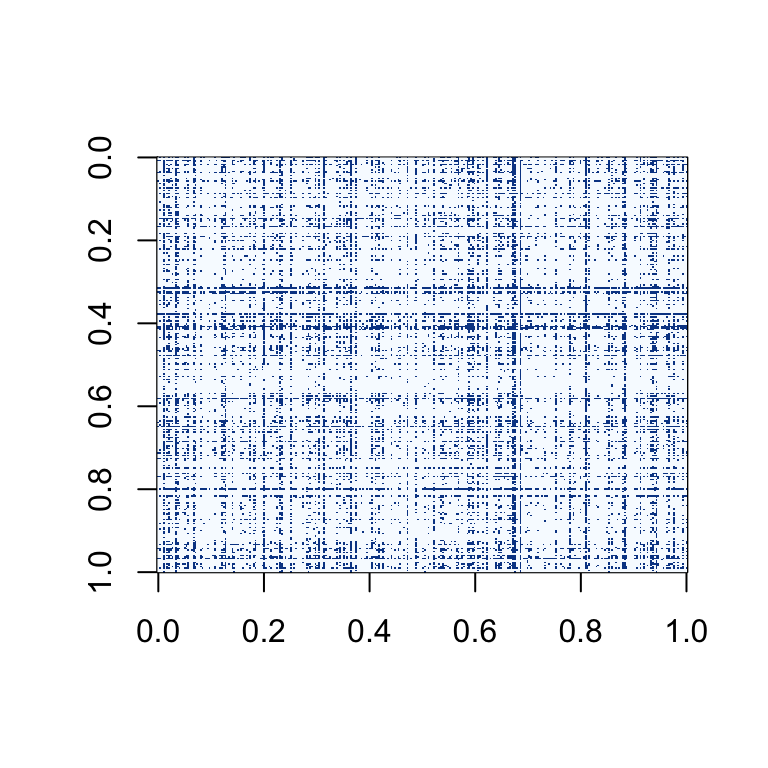
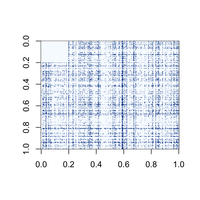
The matrix below is one of the ten sampled matrixes without any modifications. This data is sampled from the generative model described above.The dark blue squares indicate that there is a relationship between two nodes and then the light blue squares represent the lack of a relationship between two nodes.

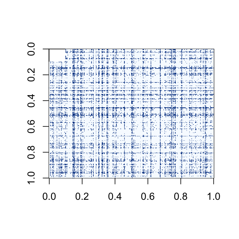
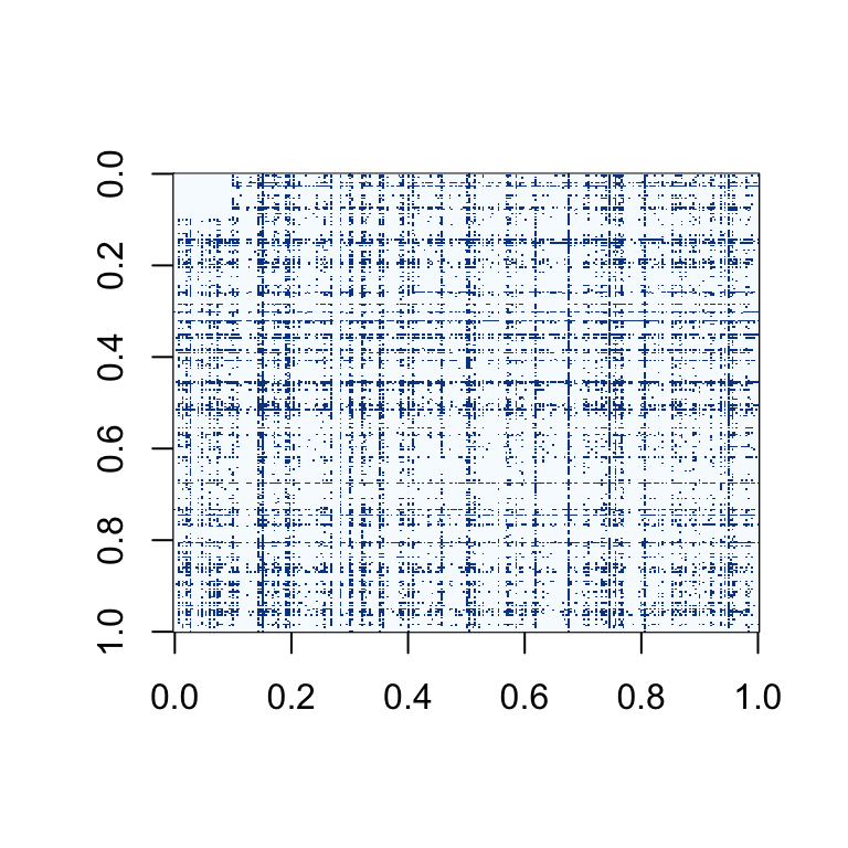
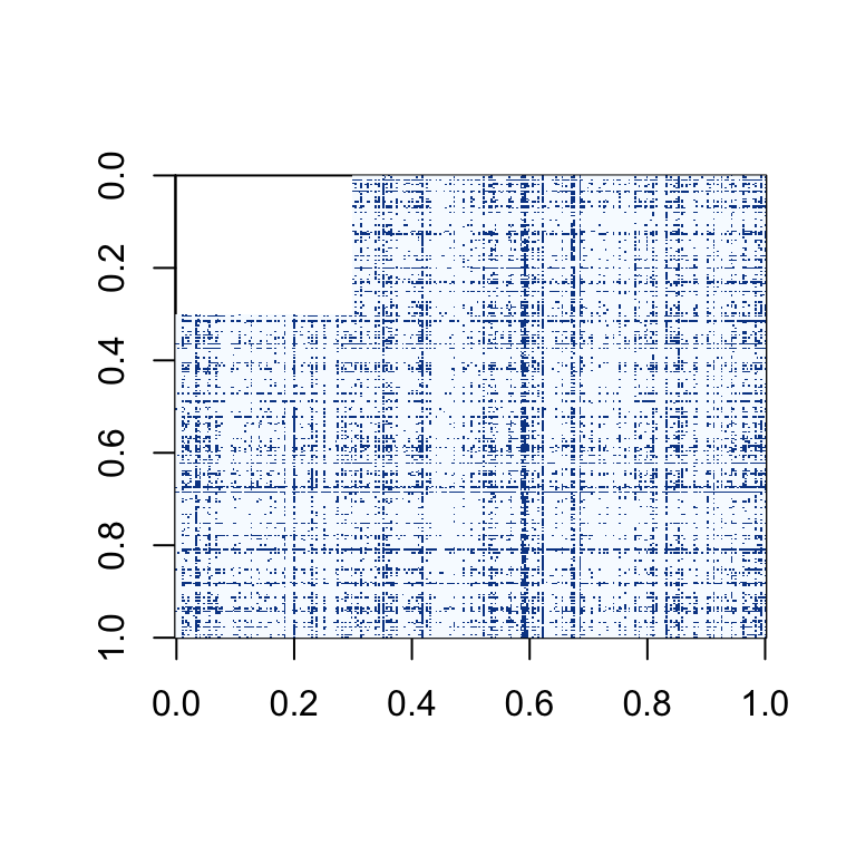
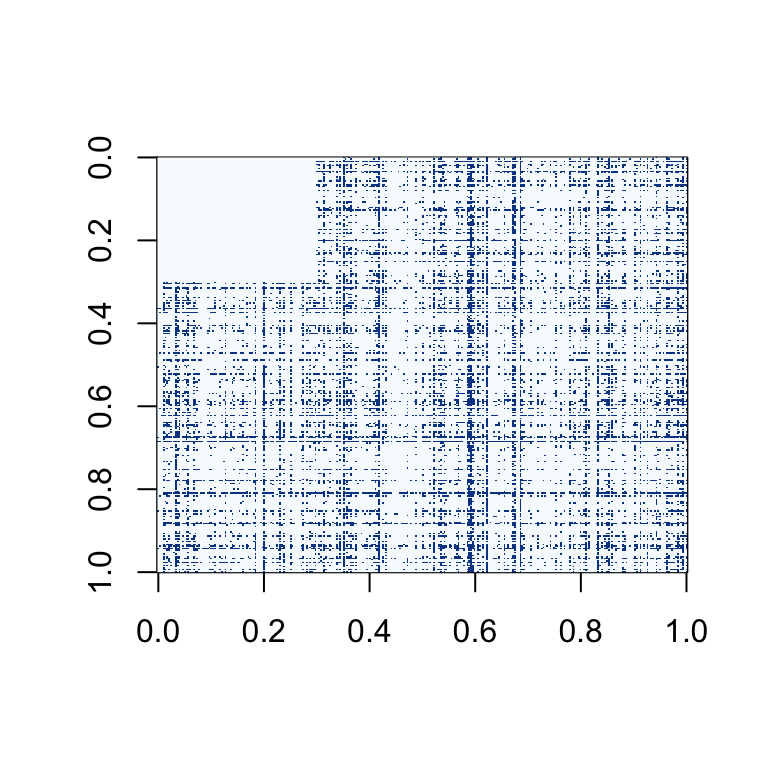
The two matrices below have been modified from the original sampled matrix. The matrix on the left has 10% of the entries replaced with NAs, this is indicated by the white square in the left corner. The matrix on the right has 10% of the values replaced with 0s.

These two matrices have the same modifications as above, but the proprtion of NAs and extra 0s in the matrix is 20%.

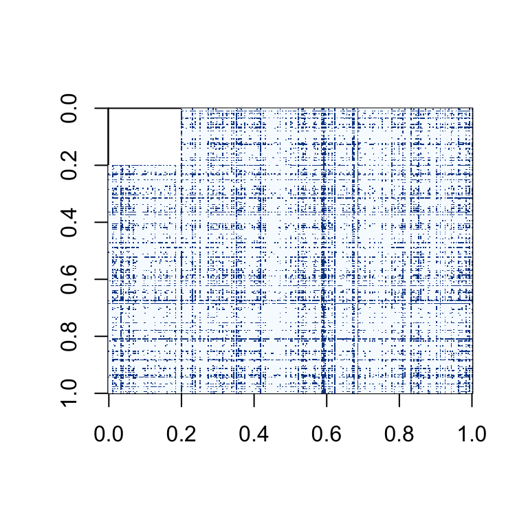
These two matrices have the same modifications as above, but the proprtion of NAs and extra 0s in the matrix is 30%.

3.1.2 Exploratory Data Analysis

Before running social network models on the observed and corrupted data, a brief exploratory data analysis was completed. The graphs may give us an indication of what we expect the posterior distributions to give us.

3.1.2.1 Degrees

All-degree

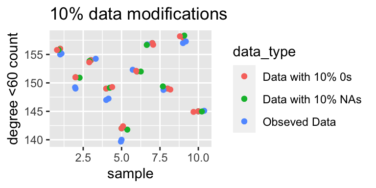
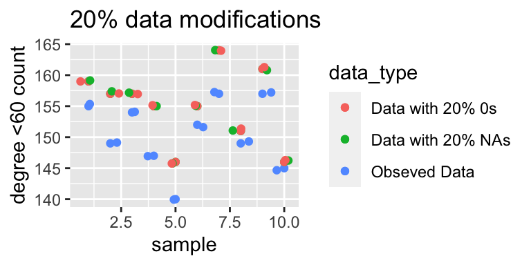
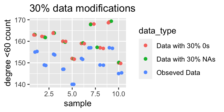
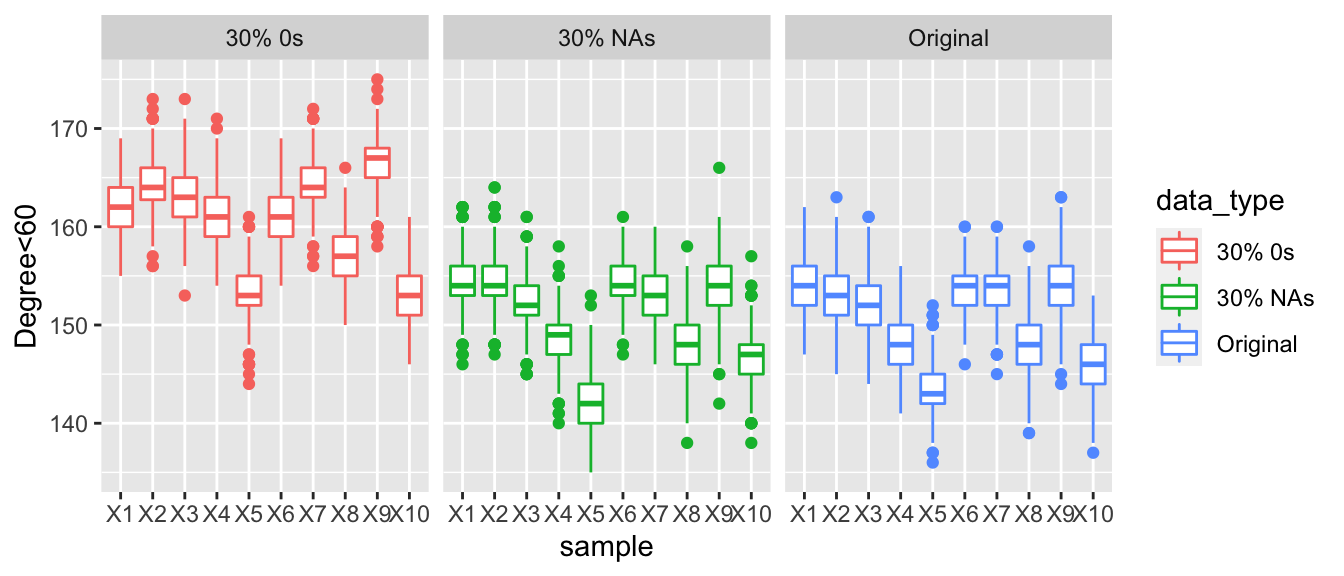
The graph below displays the number of actors with total degrees less than 60, across 10%, 20% and 30% replacements with NAs or 0s. As we increase the proportion of corrupted data there is a clear gradual widening in the difference between the values of the number of nodes with a degree less than 60. In the first graph all the three points for each sample are very similar but as we increase the amount of corrupted data the gap widens.

In-degree

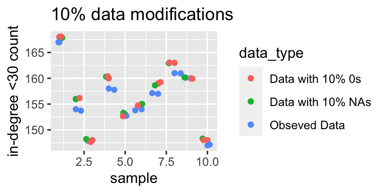
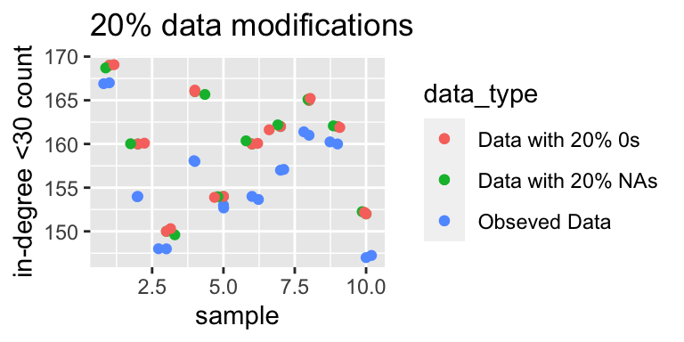
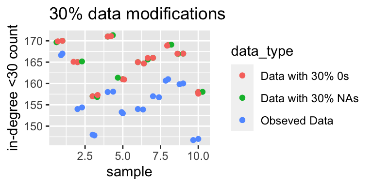
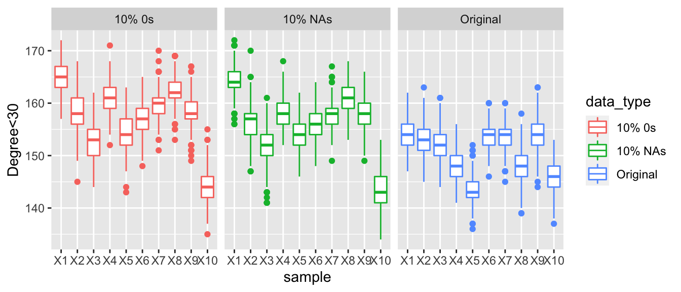
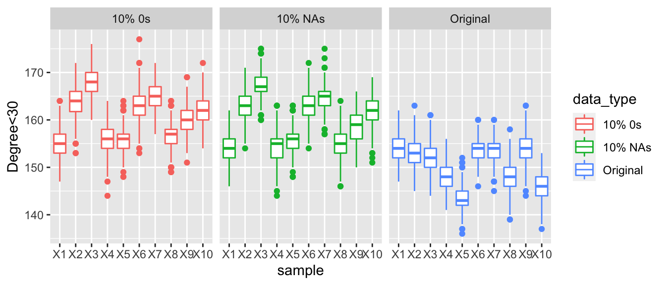
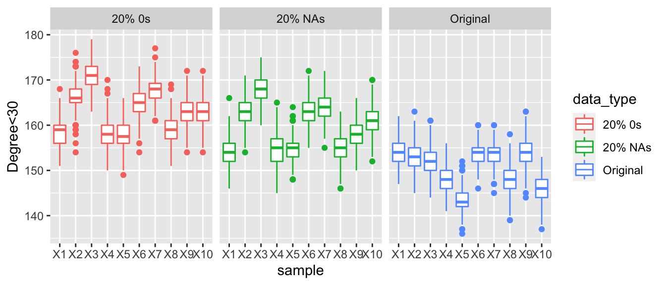
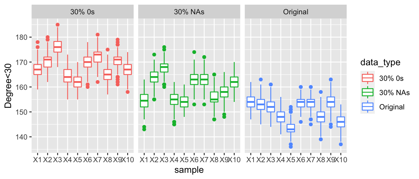
The graph below displays the number of actors with an in-degree less than 30. There is a very similar trend as above, indicating that for some actors their popularity appears to be decreasing.

Out-degree

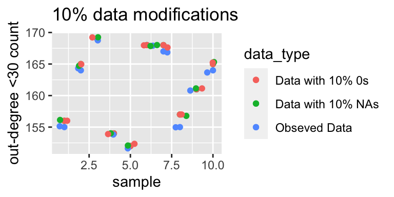
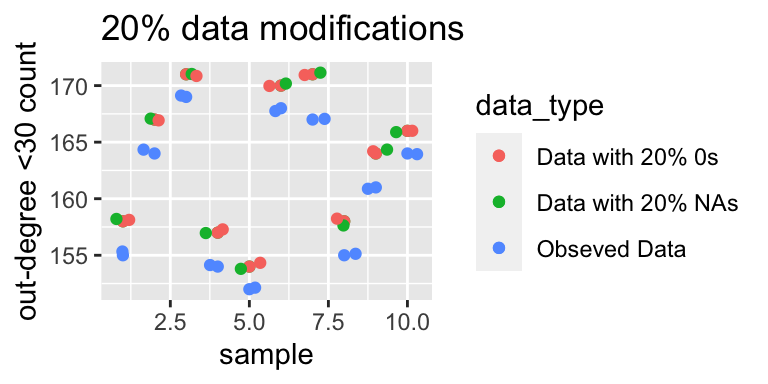
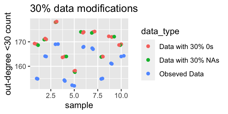
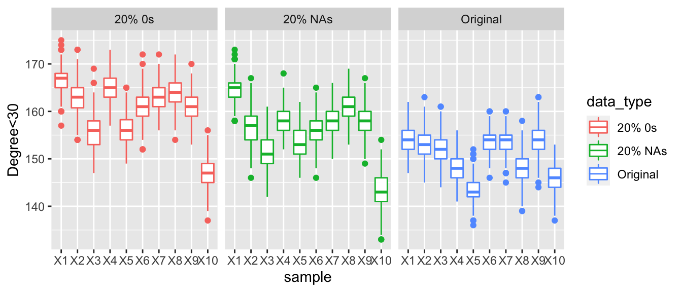
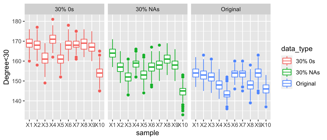
The graph below shows the number of actors with an out-degree less than 30. Again, the trend is very similar to the above two, but this also indicate that for some actors their sociability also appears to be decreasing.

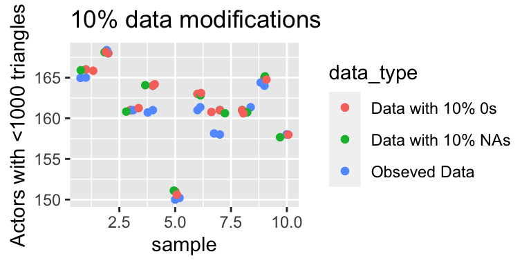
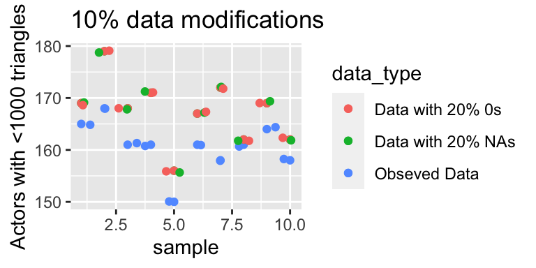
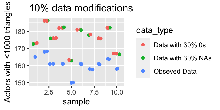
3.1.2.2 Count Triangles

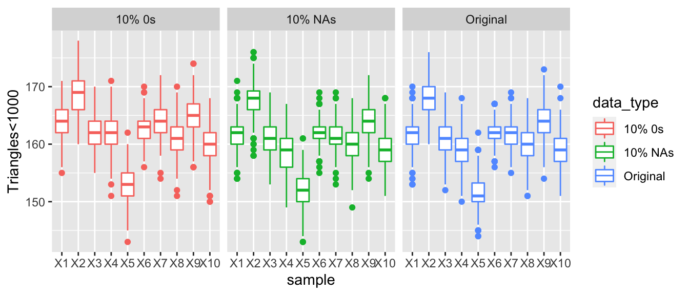
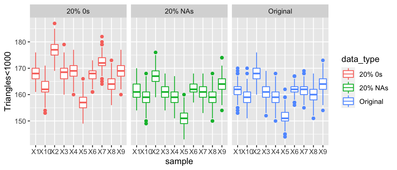
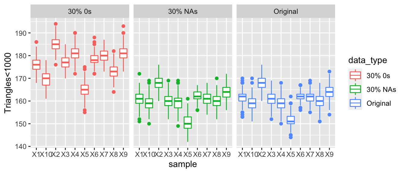
The graph below represents the number of nodes that have a triangle count of less than 1,000. Thus, as the number of nodes that have a triangle count of less than 1,000 increase this demonstrates that the graph may be becoming more disconnected and have fewer transitive properties. The graph on the right represents the original data, the data replaced 10% with NAs and 10% with 0s. All dots appear to be relatively similar and there are no large differences between the three datasets. However, if we increase the proportion of 0s and NAs in our data to 30% then we see that there is a growing difference between the number of nodes that have a triangles count of less than 1000 compared, where as we increase the number of 0s or increase the amount of corruptness in the data the values of our summary statistics stray further from the values of the full observed data.

3.1.4 Findings

3.1.4.1 Coefficients

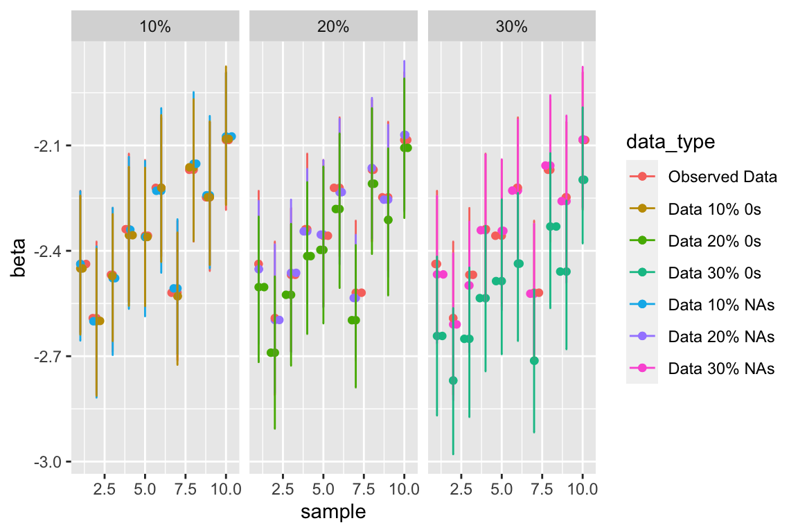
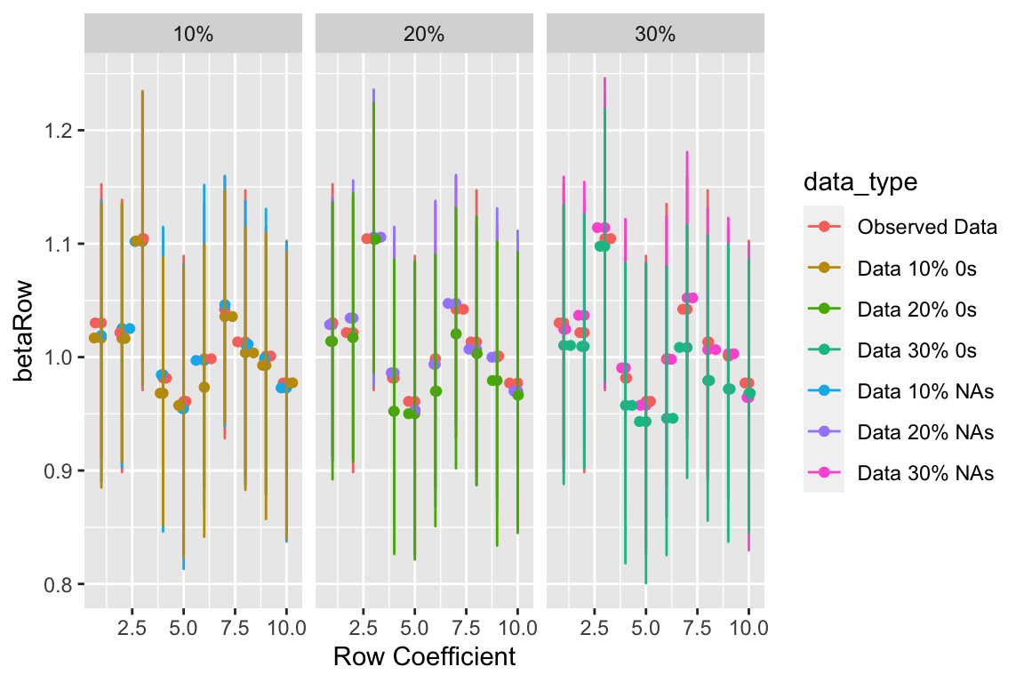
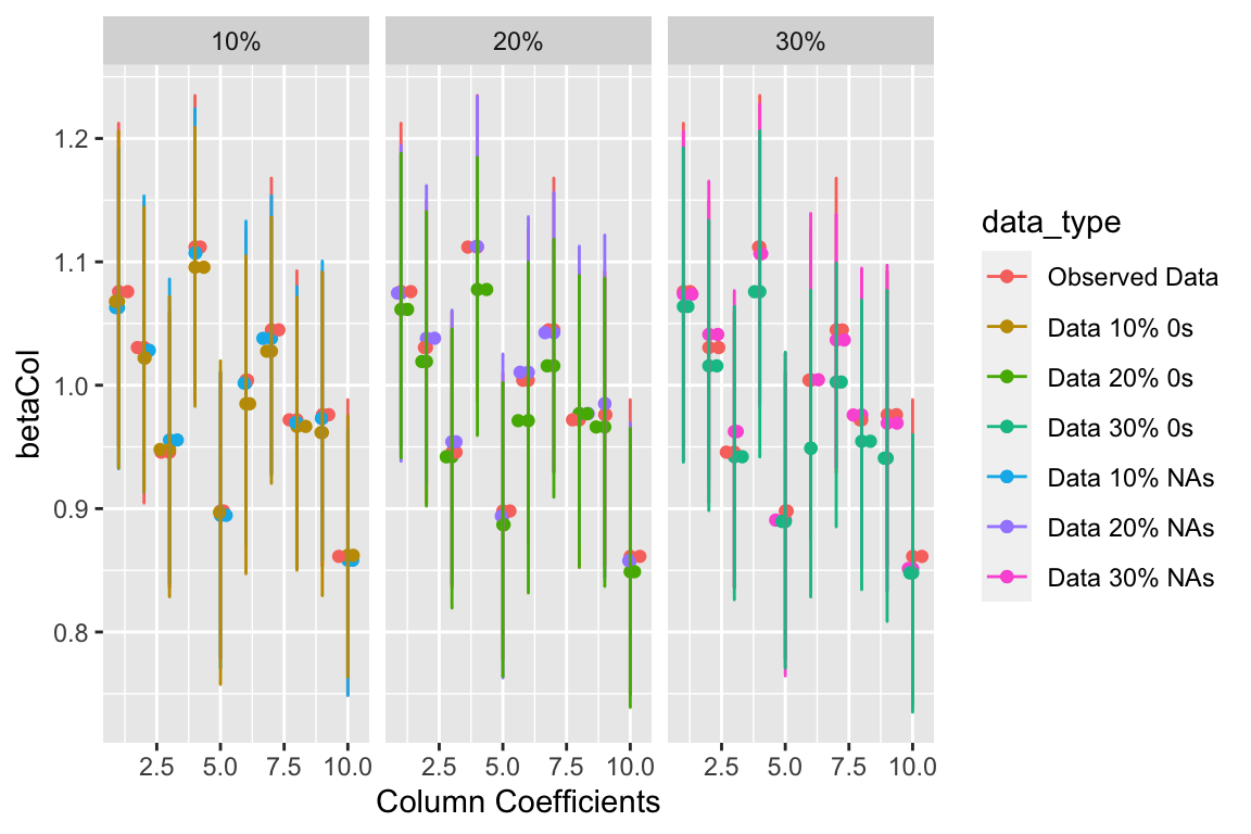
We predict that as the percentage of 0s within the data increase, the intercept will be pulled down and the row and column coefficients will be pulled closer to zero, further from their true value of 1. We also hypothesized that as we increase the number of NAs, it will increasingly become more difficult to accurately estimate the value of the true coefficient but should still be similar. As expected, that data that had a proportion of NAs, though the credible intervals are a wider than the full observed data, the estimates of the coefficients remain very closely aligned with the full data. Providing support for our hypothesis that NAs will not impact the inference but have greater uncertainty around the inference. This trend is continued throughout the following posterior-predictive summary statistics. This implies that as the number of countries who are reporting false arms trade are increasing then the intercept for our model may be pulled down. This trend is present for the column and row means as well. As the number of countries under reporting their data increases then the coefficients for the row and columns get pulled down farther from the estimates of the NA and the observed data.

Intercepts

Row Coefficients

Column Coefficients

3.1.4.2 Degree Distribution

All-degree

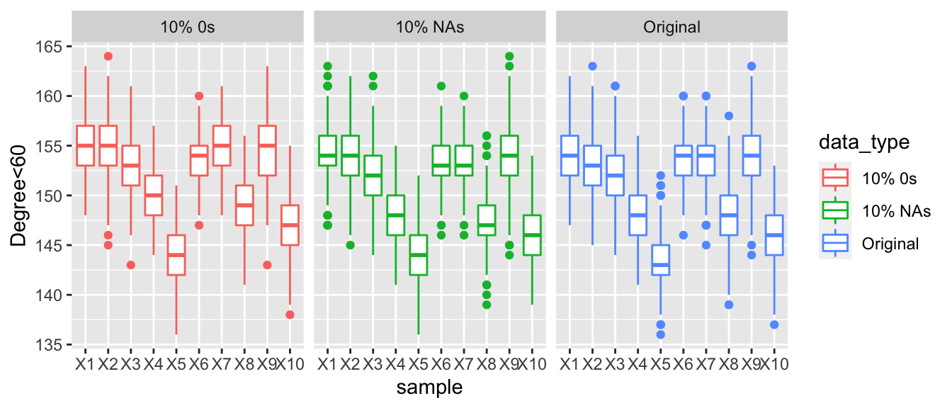
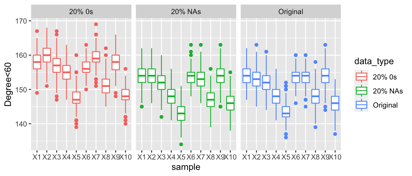
Here we are looking at the posterior predictive values for the number of actors with a total degree of less than 60. When comparing the three graphs, there is a clear trend as we increase the number of countries who are under reporting their arms trade the number of degrees that are under 60 increases. Looking at the graphs when 30% of the values are corrupted then the boxplots are much higher than those of the observed data and the data with NAs. Make not that even with 30% of the values in the data being replaced with NAs that the degree distribution appears to be very similar to the observed data.

In-degree

A similar trend as above is shown as the number of degrees under 30 increases, demonstrating that some actors are appearing not as popular the more corrupted is present.

Out-degree

The number of degrees out-degrees under 30 increases showing that some actors are appearing less sociable as the amount of corrupted data increases.

3.1.4.3 Counting Triangles

Analyzing the graphs over the varying proportions of NAs and 0s, we see that as the number of 0s increases there are a larger portion of nodes that are a member of less than 1000 triangles. This demonstrated that the graph grows increasingly less connected and might have altered some of the clusters originally present. It’s also important to note that the data that had a proportion replaced with NAs is very similar to the original distribution, this is in line with our initial hypotheses. Since the missing values are being imputed from the generative model, we would expect their inference to be close to the original samples.

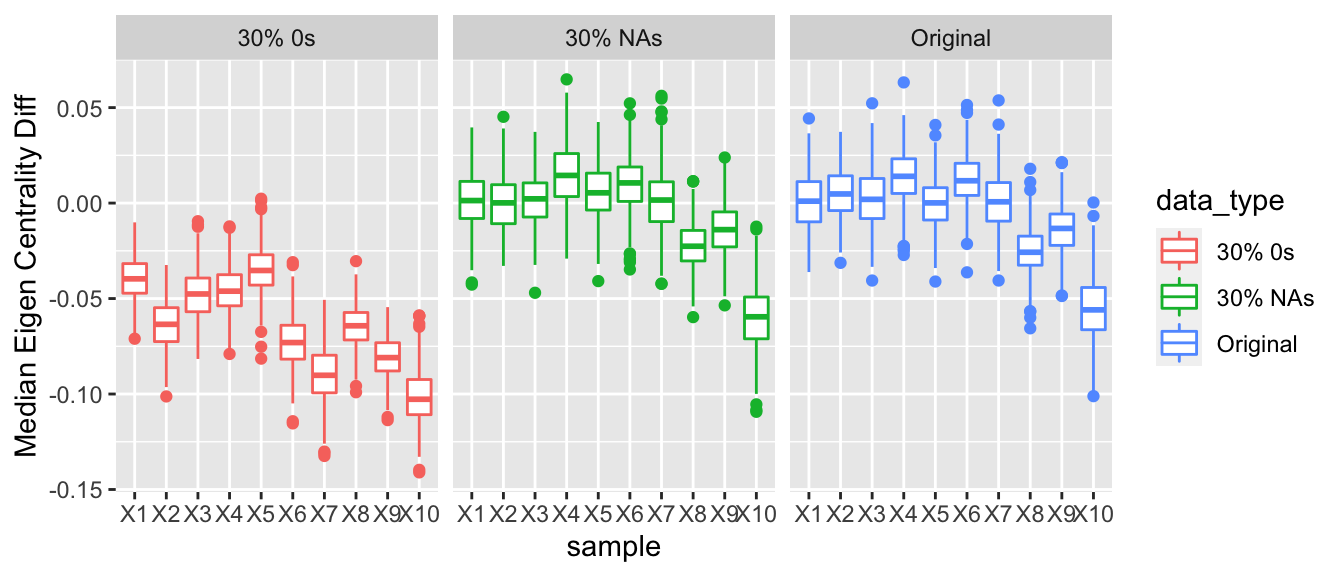
3.1.4.4 Eigen Vector Centrality

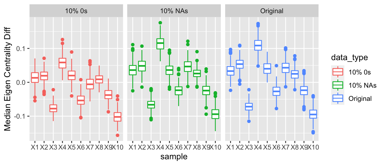
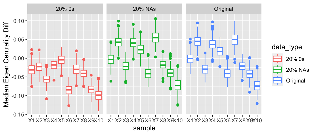
For nodes that are underreporting their arms, they will have fewer relations and thus appear not as important or influential to the network as they might be. Thus, nodes that are underreporting may tend to have a lower eigen vector centrality than nodes that are reporting all their arms trades. To get at this difference we took the three types of data we had: the observed data, the data with a proportion of NAs, and then the data with a proportion of 0s. Then we looked at the posterior predictive eigen vector centrality for the nodes at each iteration in the Gibbs sampler. The median eigen vector centrality for the nodes that were considered to be underreporting was calculated and then the median eigen vector centrality for the rest of the nodes was calculated. The difference of these two values was then computed. Thus, for the observed data and for the data with a proportion of NAs we would not expect there to be any difference for the distributions of the difference in medians to be centered at 0. However, for the data where we inserted a proportion of 0s, we would expect the median eigen vector centrality for the nodes that were underreporting their arms trade to be less than the eigen vector centrality for the rest of the nodes who are accurately reporting their data.

This result was observed, and as we increased the proportion of nodes that are underreporting, we see that the difference between the median eigen vector centrality of the nodes that are underreporting also decreases and the nodes that were reported accurately increased.

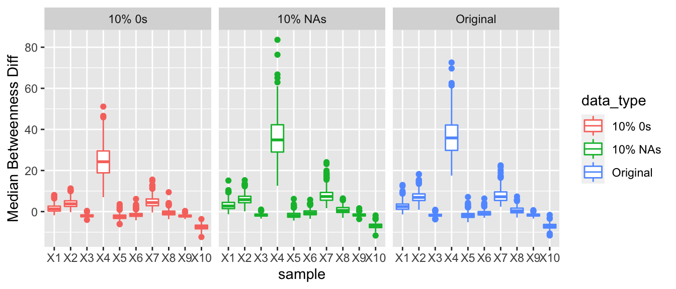
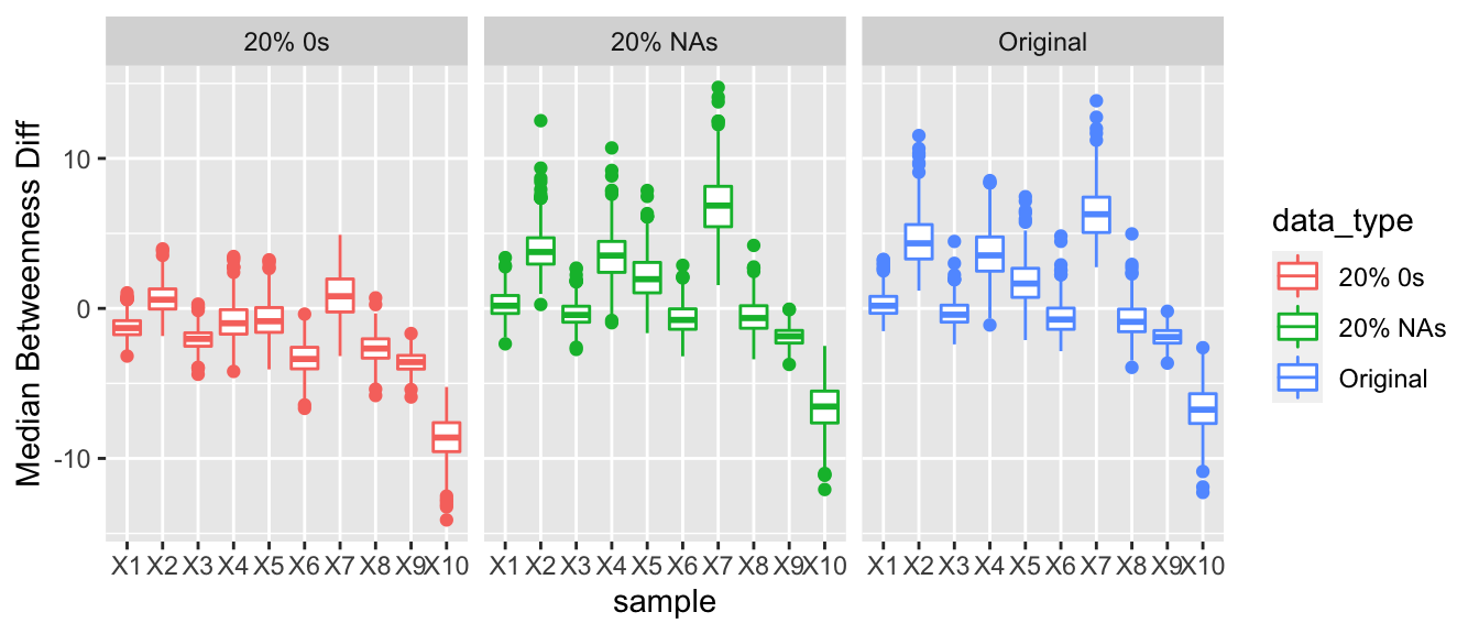
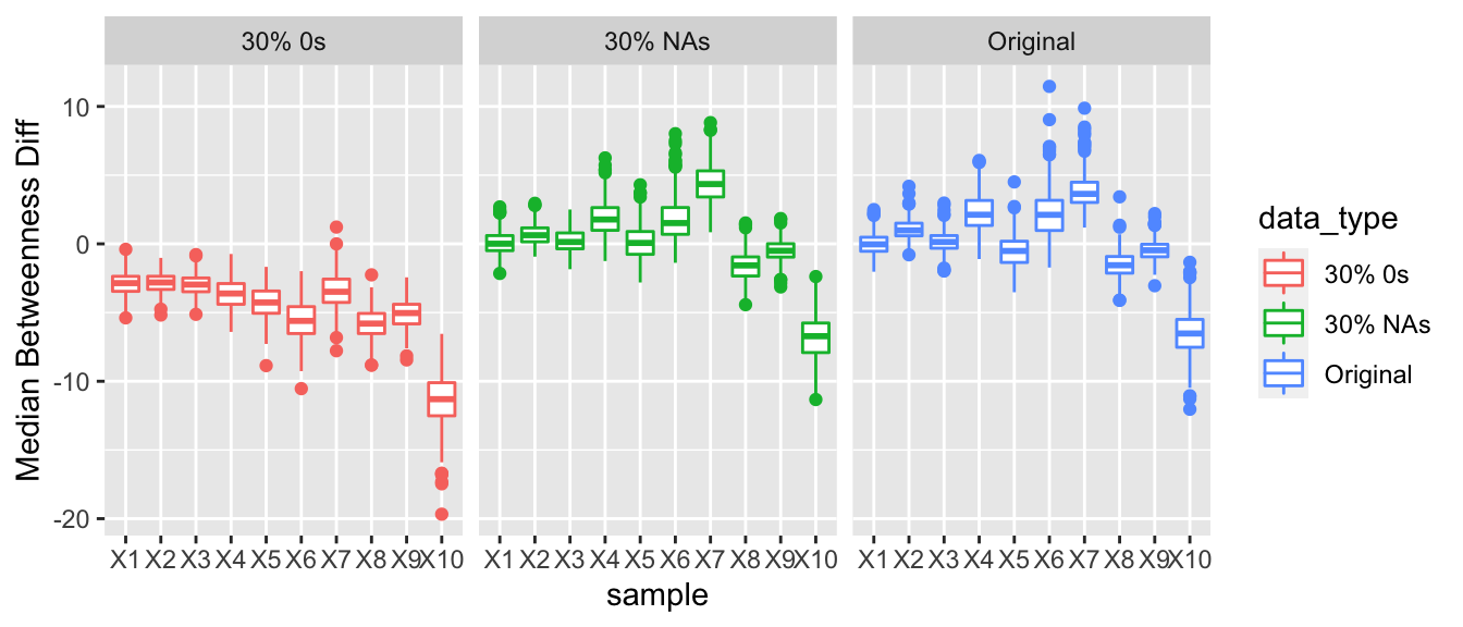
3.1.4.5 Betweenness

For betweenness we hypothesized that the nodes that were not reporting their full arms trade would have a lower betweenness score than countries that were reporting their full arms trade. Similar to eigen vector centrality we would expect for nodes that underreported their arms, their median betweenness score would be less than the nodes who reported their full arms trading. This trend was observed, and as the proportion of 0s was increased the difference between the median betweenness of the nodes underreporting and the nodes that were accurately reporting increased.

3.2 Hypothesis Testing

Though the posterior predictive distributions above show a visual difference in the distributions between the three data types, we wanted to quantify this difference. When carrying out analyses with small arms data that may be corrupted, the main question that we are trying to address is are the data that have been replaced with a percentage of 0s coming from the same distribution as the original sampled data, in other words, is \(Y_{0}\) coming from the same distribution as \(Y_{obs}\)? We designed a hypothesis test to examine this question, the following method was taken:

To get the null distribution, we sampled 1,000 data sets from the original generative model.
The test statistics for each distribution was then calculated (number of actors with total-degrees less than 60, number of actors with in-degree less than 30, number of actors with out-degree less than 30, number of actors with a triangle count of less than 1,000).
We then examined the posterior predictive distribution of \(Y^{obs}\), \(Y^{NA}\), and \(Y^{0}\) for each of the 4 summary statistics. The following questions are:

In this resampled graph, do I have more nodes with a degree fewer than 60, than one would expect under the null distribution?
In this resampled graph, do I have more nodes with a triangle count fewer than 1,000, than one would expect under the null distribution at each iteration?

Then the posterior predictive p-value is calculated with respect to the empirical distribution of the count of triangles that equal 0 or 1. \(P(T>T^{obs} | the null)\).

The posterior predictive p-value represents a measure of discrepancy between the null value and the sampled data.

3.2.1 Hypothesis Testing Findings

3.2.1.1 Degrees

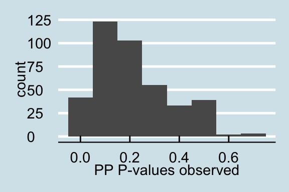
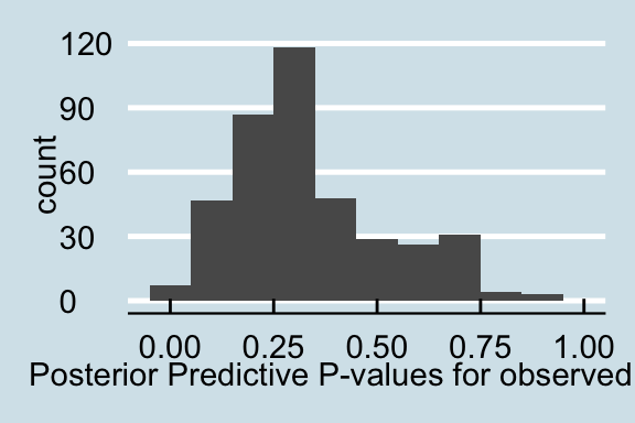
After completing the above algorithm for computing posterior predictive p-values these values are plotted in order to see the distribution of the posterior predictive p-values. If we initially consider the posterior predictive p-value distribution for the original data, then we see that only a small number of the samples are getting rejected (are less than .05). A similar trend is present when looking at the data that originally had a proportion of values replaced with NAs. This is what one should expect as these missing values are being imputed from the generative model. This demonstrates that even if there are high levels of corruption in the data that replacing theses values with NAs will allow the inference to remain relatively unaffected when considering the number of total-degrees under 60.

Posterior Predictive P-values for the observed data

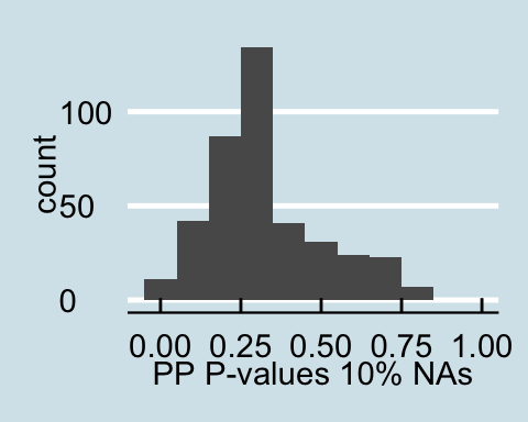
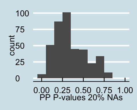
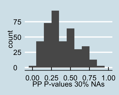
Posterior Predictive P-values for data with a proportion of NAs

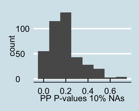
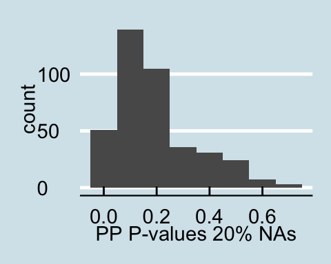
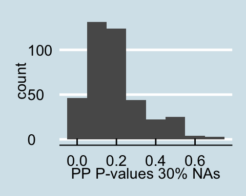
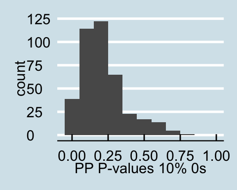
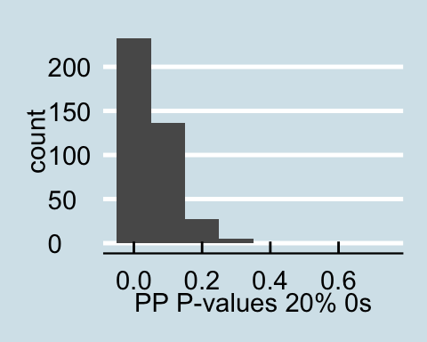
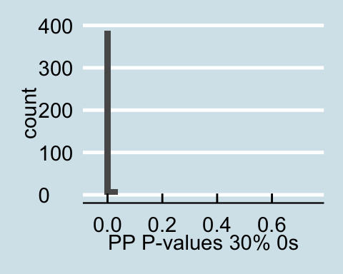
Upon examining the data that has a proportion of zeros, we see that as the amount of corrupted data increases the posterior predictive p-values all become less than .05 signifying that for all values in the posterior predictive distribution, the distribution of the number of actors with degrees under 60 is different from the null distribution. Similar trends are found for in-degree and out-degree descriptive statistics.

Posterior Predictive P-values for data with a proportion of 0s

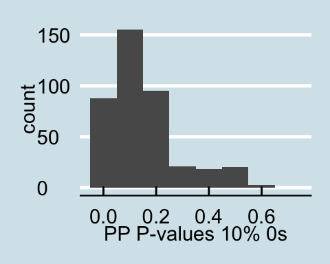
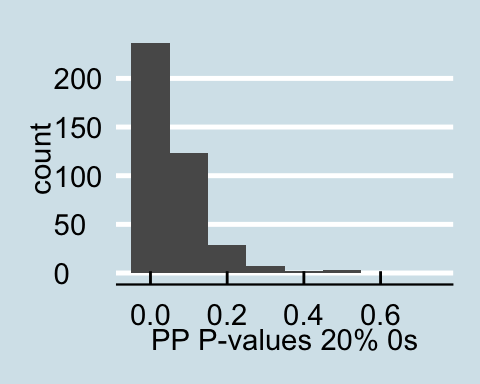
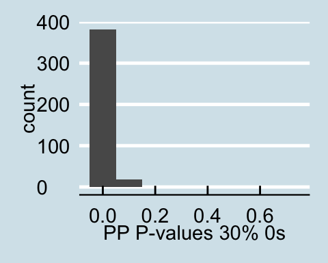
The graphs above present the results of one sampled dataset out of the 10 that we initially sampled from the generative model, but the trend is the same throughout all 10 samples.

3.2.1.2 Count Triangles

A similar trend as above is found for counting triangles. The posterior predictive p-values generated from the data with a proportion of the values replaced with NAs is very similar to the distribution of p-values form the full observed data. However, increasing the proportion of corrupted data lead to the posterior predictive distribution of actors with a triangle count of less than 1000 that is different from the null distribution, demonstrated by almost all of the p-values being less than .05.