Chapter 5 Equations & Inequalities

5.1 Introduction

Consider the following statements:

$4 > 8$ (“4 is greater than 8”)
$4 < 8$ (“4 is less than 8”)

The first statement is false. The second statement is true.

A statement like:

$x>8$

is an “open” statement, if x is not known. x is called a variable.

4>8

## [1] FALSE

4<8

## [1] TRUE

5.2 Solving Equations with One Variable

Rule 1: x + z = y + z, if x = y

Equations, that is, are equivalent when adding the same number to the left hand and right hand sides of the equal-to (“=”).

Rule 2: xz = yz, if x = y

Remember that $xz$ is short for $x*z$, or in words, x times z.

Equations are equivalent when multiplying the left hand and right hand sides by the same number.

Below, we assign the value 3 to both $x$ and $y$. Obviously, $x=y$. Next, we multiply both $x$ and $y$ by the same number $z=2$. Since $x=y$, $xz=yz$.

We use an if/else statement to evaluate whether $x$ and $y$ are the same. The cat() function prints the output.

x<-3
y<-3
z<-2
xz<-x*z; yz<-y*z
if(xz == yz){
cat("Yes, xz=yz!!")
} else {
cat("Nope, they differ")
}

## Yes, xz=yz!!

x<-4
y<-3
z<-2
xz<-x*z; yz<-y*z
if(xz == yz){
cat("Yes, xz=yz!!")
} else {
cat("Nope, they differ")
}

## Nope, they differ

Using these transformation rules we can solve equations.

For example:

$2x + 5 = 10$

subtract 5, from both sides of the equation:

$2x + 5 - 5 = 10 - 5$

$2x = 5$

divide both sides by 2:

$2x/2 = 5/2$

$x = 2.5$

Check for yourself:

$3x + 5 = x - 1$

Answer: x = -3

$(x + 2)/5 = 3$

Answer: x = 13

5.3 Linear Inequalities

Rule 1:

$x + z > y + z$, if $x>y$

$x + z < y + z$, if $x<y$

Rule 2a (z>0)

$xz > yz$, if $x>y$

$xz < yz$, if $x<y$

Rule 2b (z<0)

$xz > yz$, if $x<y$

$xz < yz$, if $x>y$

Let’s use R to illustrate these rules.

In the example below, $z$ is a positive number. If $x<y$ is true, then the claim is that after multiplying both sides by $z$, the result is still true.

# Example (rule 2a)
z=2
x=3
y=4
x<y

## [1] TRUE

z*x < z*y

## [1] TRUE

You see that the inequality still holds when multiplying both sides by a positive number.

But if $z$ is a negative number, then things change!

While $x<y$ (indeed, $3<4$!), multiplying $x$ and $y$ by the same negative number reverses the sign: $z*x>z*y$ (as $-2*3 >-2*4$, or $-6>-8$).

Using the same values for $x$ and $y$ as above, but using $z=-2$, we will get the following.

# Example (rule 2b)
z=-2 # z now is a negative number!!
x=3
y=4
x<y

## [1] TRUE

z*x < z*y

## [1] FALSE

(x<y) == (z*x < z*y) # Are both statements either TRUE or FALSE (!) ??

## [1] FALSE

The inequality no longer holds when multiplying both sides by a negative number.

Or, to put it differently, the sign reverses, from “smaller than ($<$)” to “larger than ($>$)”.

Check for yourself:

$-x + 1 > 6$

Answer: x < -5

A slightly more complicated expression is the following. Here, we have two inequalities in one statement. Basically it says that $-x$ is in between $-8$ and $-5$. But what does that mean for $x$?

$-8 < -x < -5$

Answer: 5 < x < 8

Just follow the rules: multiply by -1 to get $x$. That will reverse the signs, from $<$ to $>$. Or: $8 > x > 5$.

x, that is, is a number in between 8 and 5.

Since our line of numbers runs from small to large, it is more common to state that x lies between 5 and 8 (x is larger than 5 but smaller than 8). If $8>x$, then $x<8$ (applying all the rules)! And if $x>5$, then $5<x$. Cosmetically, it looks nicer. But mathematically speaking, there’s no difference.

5.4 Equations with Two Variables (or “Unknowns”)

Consider the following pair of equations:

[1] $x = y + 4$

[2] $x = 0.5*y - 3 $

Rather than a line of numbers, we now have two dimensions. The relations represent lines in a two-dimensional space. As long as the lines do not run parallel to one another, there must be one single combination of values of $x$ and $y$ where the lines meet.

One method of solving linear equations is by “substitution”.

The first equation already provides an expression for $x$, in terms of $y$. Otherwise, we could use the transformation rules to obtain such an expression.

Substituting $x$ [1] in [2], we get:

$y + 4 = 0.5y - 3$

And using the rules of transformation:

$0.5y = -7$ (subtract $0.5y$ from both sides; subtract 4 from both sides)

Hence: $y = -14$ (multiply both sides by 2)

and: $x = -14 + 4 = -10$

This method can be extended to sets of 3 equations and 3 variables, or in general to sets of n equations and n variables.

As you can imagine, it will get increasingly tedious and error prone to find the solutions for all variables!

5.4.1 The matlib package

Luckily, you can make use of the matlib package in R, and make use of the functions of matlib.

# install.packages("matlib")
library(matlib)
A <- matrix(c(1,1,-1,-.5),2,2)
b <- c(4,-3)
showEqn(A,b)

## 1*x1   - 1*x2  =   4 
## 1*x1 - 0.5*x2  =  -3

plotEqn(A,b)

## x[1]   - 1*x[2]  =   4 
## x[1] - 0.5*x[2]  =  -3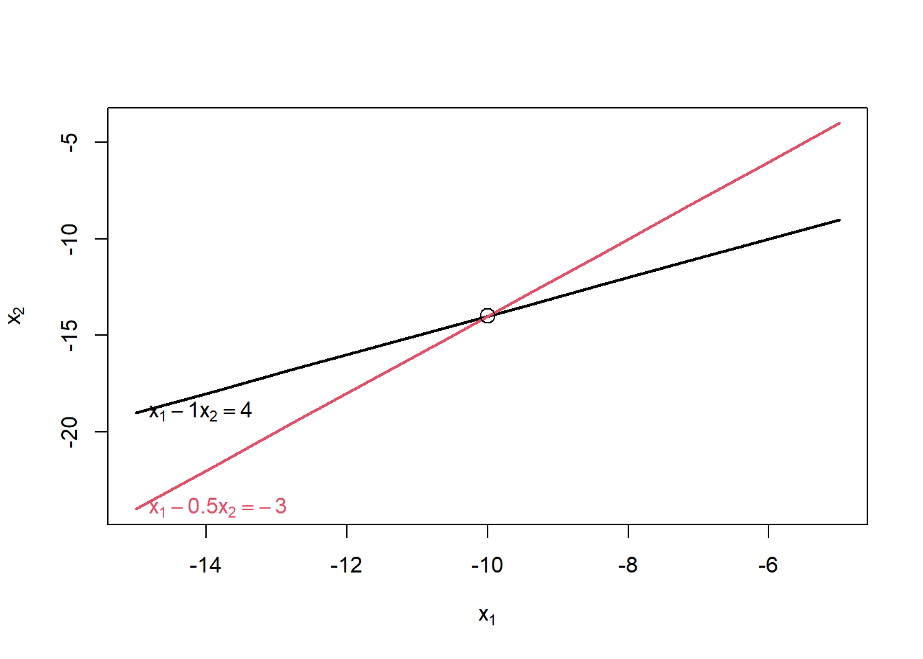

Solve(A,b,fractions=TRUE)

## x1    =  -10 
##   x2  =  -14

Let’s inspect these lines of code, step-by-step.

We first invoke the functions in the matlib package, using the library() function. Before doing so, see to it that you have installed the package. In RStudio, check the Packages installed in the user library.

We then define a 2*2 matrix containing the coefficients of the equations on the left hand side. Note that the equations have to be rewritten in the format:

$c1*x + c3*y = b1$

$c2*x + c4*y = b2$

In our case, we have:

$x = y + 4$, to be rewritten as:

$x-y = 4$, for the first equation.

And:

$x = 0.5y - 3$, to be written as:

$x -0.5y = -3$, for the second equation.

Summarizing:

$x-y = 4$

$x-0.5y = -3$

In our case, the 4 coefficients are then 1, 1, -1 and -0.5, for $c1$ to $c4$ respectively. Use the correct order, from $c1$ to $c4$!!

The first value (1) is the coefficient ($c1$) of the first variable ($x$) in the first equation.

The second value (1) is the coefficient ($c2$) of the first variable ($x$) in the second equation.

The third value (-1) is the coefficient ($c3$) of the second variable ($y$) in the first equation.

And the fourth value (-0.5) is the coefficient ($c4$) of the second variable ($y$) in the second equation.

The numbers 2 and 2 in the matrix() functions indicate the number of columns and rows.
The coefficients b are 4 and -3.
The showEqn() function allows you to check if the implied equations match the ones you want to solve. You can use the plot(Eqn) to see what the lines look like, in the two-dimensional space.
The Solve() function gives the results for x and y (although the software uses x1 and x2).

As an example, and to get some practice, adapt the above to find x and y for the following set of equations:

$3x + 5y = 11$

$2x - y = 16$

library(matlib)
A <- matrix(c(3,2,5,-1),2,2)
b <- c(11,16)
Solve(A,b,fractions=TRUE)

## x1    =   7 
##   x2  =  -2

There are two special cases.

The first case is the existence of identical lines, as in:

$3x + 6y = 9$

$5x + 10y = 15$

Multiplying the first equation by 5, and the second one by 3 gives:

$15x + 30y = 45$

library(matlib)
A <- matrix(c(3,5,6,10),2,2)
b <- c(9,15)
showEqn(A,b)

## 3*x1  + 6*x2  =   9 
## 5*x1 + 10*x2  =  15

plotEqn(A,b)

## 3*x[1]  + 6*x[2]  =   9 
## 5*x[1] + 10*x[2]  =  15

Solve(A,b,fractions=TRUE)

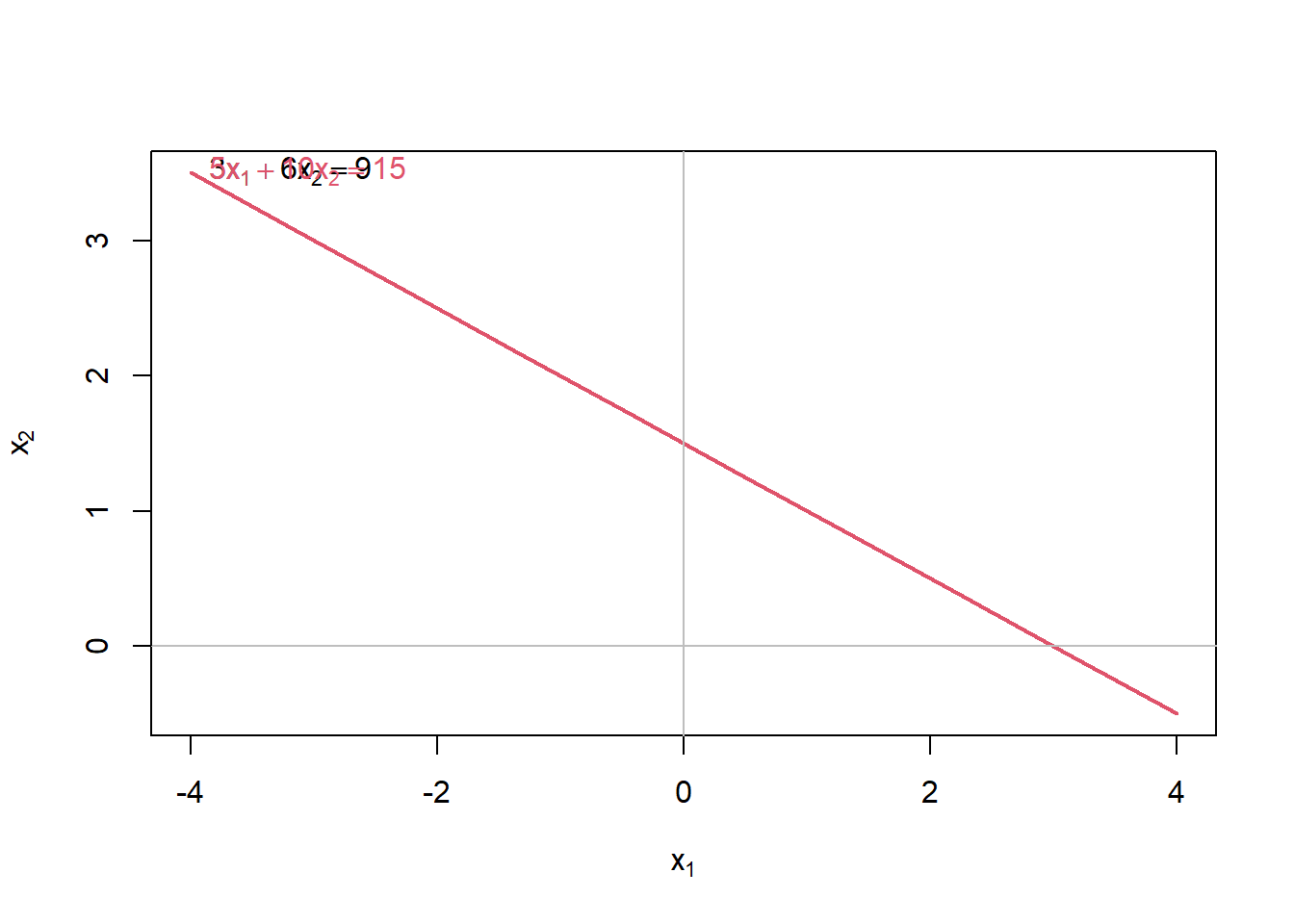
## x1 + 2*x2  =  3 
##         0  =  0

The plot produces, indeed, one thick line, representing both equations.

The two equations are identical, and produce the same line. The two equations are always true regardless of the values of x and y. Or, as the output shows, 0=0; which is true regardless of x and y!

A second instance is when the lines do not coincide but run parallel. In that case there is no solution, as the lines never meet.

$2x - y = -6$

$6x - 3y = 12$

library(matlib)
A <- matrix(c(2,6,-1,-3),2,2)
b <- c(6,12)
showEqn(A,b)

## 2*x1 - 1*x2  =   6 
## 6*x1 - 3*x2  =  12

plotEqn(A,b)

## 2*x[1] - 1*x[2]  =   6 
## 6*x[1] - 3*x[2]  =  12

Solve(A,b,fractions=TRUE)

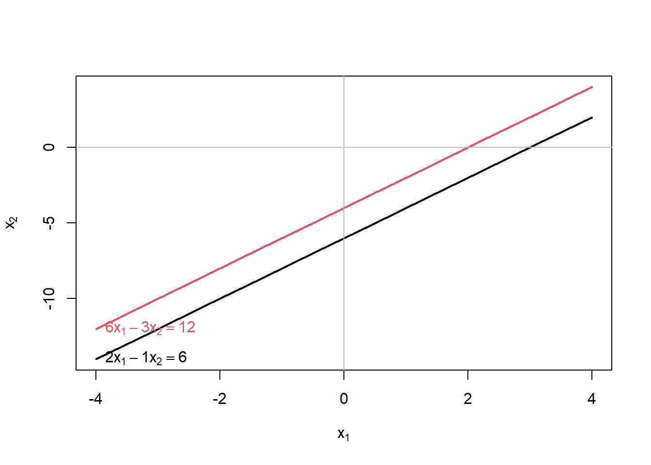
## x1 - 1/2*x2  =  2 
##           0  =  2

The solution reads 0=2, which is never true. A bit of a cryptic way to state that no solutions for x and y can be found that solve the set of equations.

5.5 Quadratic Equations

Quadratic equations have the form:

$a*x^{2} + b*x + c = 0$

The trick to solving this equation is based on the following notion. We are going to dig back in your (hopefully not long forgotten) high-school mathematics.

Suppose that we start from:

$(x+p)*(x+q)= 0$

This expression is true if either $x=-p$ or $x=-q$. If $x=-p$, then the first part of the equation is zero, and any number times zero gives zero. Likewise, $x=-q$ would have the same effect.

For $x$ ≠ $-p,-q$, the left hand side of the equation implies multiplication of two non-zero numbers, which gives a non-zero outcome (and hence, the equality doesn’t hold).

The equation can be rewritten as:

$(x)*(x+q) + p*(x+q)= 0$

$x^{2} + (p+q)*x + pq$

Since $(x+p)*(x+q)= 0$ if one of the terms $(x+p)$ or $(x+q)$ equals zero, the trick is to find values p and q such that their sum equals b, and their product equals c.

For example, if we want to solve:

$x^{2} + 7*x + 10 = 0$

then 5 and 2 are the numbers we are looking for, since $p+q = 5+2 = 7$ and $p*q = 5*2 = 10$.

The equation then is true if $x=-2$ or $x=-5$. Check this for yourself!

We can use R-commands to plot the function, and confirm that, indeed, at $x=-2$ and $x=-5$, y takes on a value of zero.

curve(x^2+7*x+10, from=-10, to=++2, , xlab="x", ylab="y")
abline(h = 0, lty = 1)
abline(v = 0, lty = 1)
abline(v = -2, lty = 2)
abline(v = -5, lty = 2)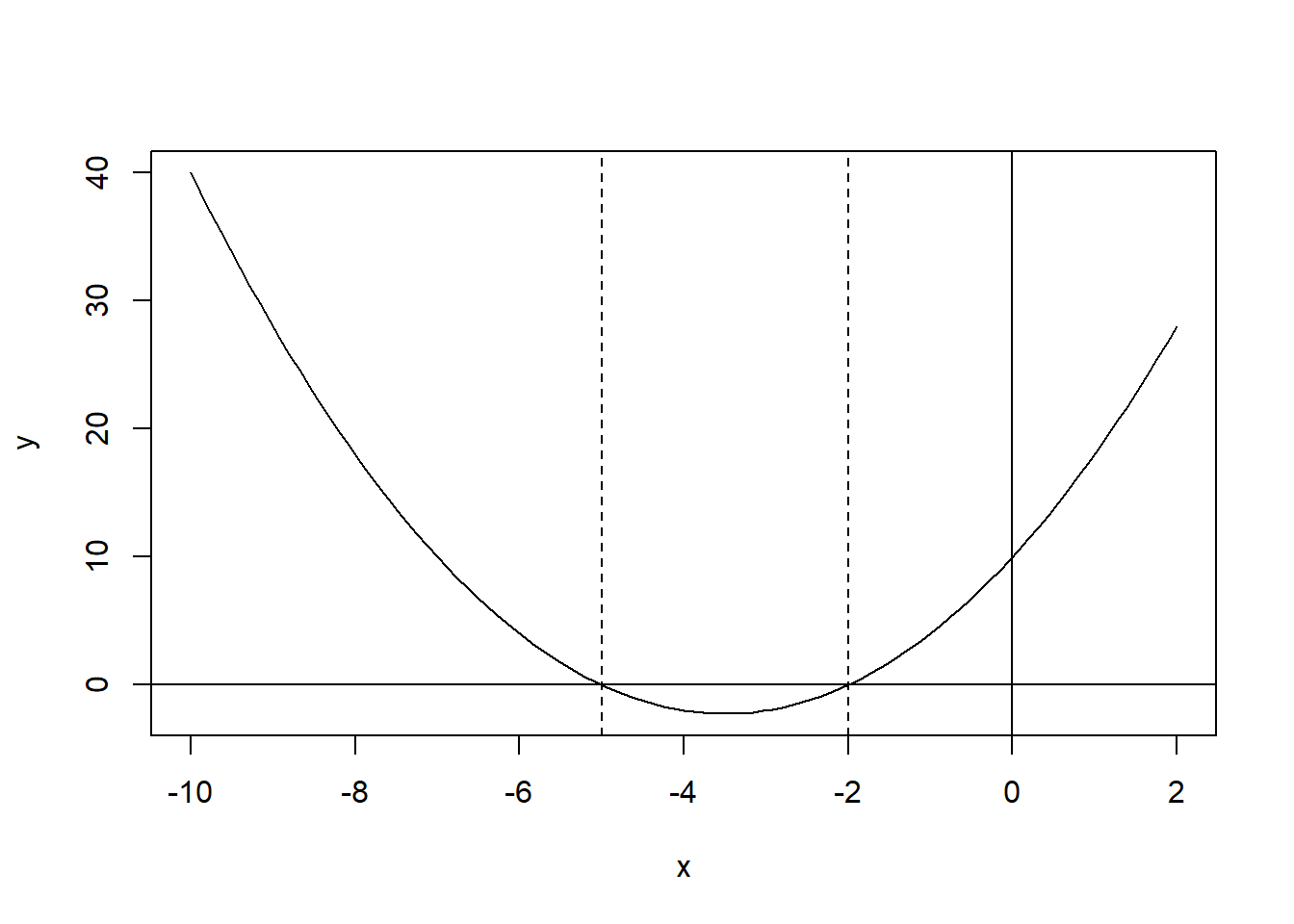

Unfortunately, it is not always easy to find the values p and q. It is better to make use of a general formula to solve the quadratic equation.

Maybe hidden at the very back parts of your brain, there’s information stored on a scary formula that you can use for solving quadratic equations.

It looks like:

\[x = {-b \pm \sqrt{b^2-4ac} \over 2a}\]

The $\pm$ reads like plus or minus, implying that this formula generates two solutions!

Some advanced R-code creates a function to easily solve any quadratic equation. We use the code written by Kiki Hatzistavrou.

It is beyond the scope of this module to explain the code below in detail. All you have to know is that:

This code defines a user-writtten function result(a,b,c) which you can use to solve your equation. The a, b and c rerpresent the coefficients in your quadratic equation.
Since R has so many users, odds are that you can find R-code for specific tasks written by somebody who has decided to share it with the rest of the world. No guarantee that it works, but most of the time it does!
If you find the code useful, store it somewhere. The code has to be run from a script, since user-written codes is not (yet) included in official packages!

result <- function(a,b,c){    # Constructing the quadratic formula
  if(delta(a,b,c) > 0){ # first case D>0
        x_1 = (-b+sqrt(delta(a,b,c)))/(2*a)
        x_2 = (-b-sqrt(delta(a,b,c)))/(2*a)
        result = c(x_1,x_2)
  }
  else if(delta(a,b,c) == 0){ # second case D=0
        x = -b/(2*a)
  }
  else {"There are no real roots."} # third case D<0
}

delta<-function(a,b,c){       # Constructing delta
      b^2-4*a*c
}

You can now use this user-written function result(a,b,c). The term a, b and c between brackets, are just the coefficients in the formula

$a*x^{2} + b*x + c = 0$

So, as an example, you can easily solve our earlier example.

$x^{2} + 7*x + 10 = 0$

using:

(result(1,7,10))

## [1] -2 -5

Solve the following examples, taken from the textbook, yourself, using the result() function.

$x^{2} = 9$

$x^{2} +4*x + 4 = 0$

$3*x^{2} + x -2 = 0$

(result(1,0,-9))

## [1]  3 -3

(result(1,4,4))

## [1] -2

(result(3,1,-2))

## [1]  0.6666667 -1.0000000

library(MASS)
fractions(result(3,1,-2))

## [1] 2/3  -1

Note that in the second example, there is only one solution: $x=-2$. Or, to put it differently, p and q have the same value (2).

By default, the formula gives the solution in decimals. We have used the fractions() function from the MASS package to give us fractions.

5.6 Exercises

5.6.1 Exercise 1

Find x for the following equations.

$42 = x+13$

$x - 3 = -12$

$12 - x = 11 - x$

$-x - 5 = -7$

$20 - (3x/5) = x - 12$

$3x - 4 > 5x$

$-3x > -x - 5$

5.6.2 Exercise 2

Solve x and y for the following pairs of equations. Use the showEqn, plotEqn() and Solve() functions to check your answers.

$7x + y = 22$
$5x + y = 14$

(Answer: $x=4$; $y=-6$)

library(matlib)
A <- matrix(c(7,5,1,1),2,2)
b <- c(22,14)
showEqn(A,b)

## 7*x1 + 1*x2  =  22 
## 5*x1 + 1*x2  =  14

plotEqn(A,b,ylim=c(-20,+20))

## 7*x[1] + x[2]  =  22 
## 5*x[1] + x[2]  =  14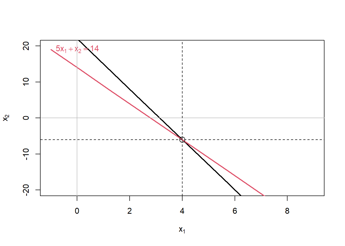

abline(h = -6, lty = 2)
abline(v = 4, lty = 2)

Solve(A,b,fractions=TRUE)

## x1    =   4 
##   x2  =  -6

$2x - y = 5$
$3x + 3y = 21$

5.6.3 Exercise 3

Solve x for the following quadratic equations:

Note that you have to write the equations in the format $a*x^{2} + b*x + c = 0$

25 - 20x + 4x² = 0

x² + 20x = -19

-4x² + 16x + 25 = 0

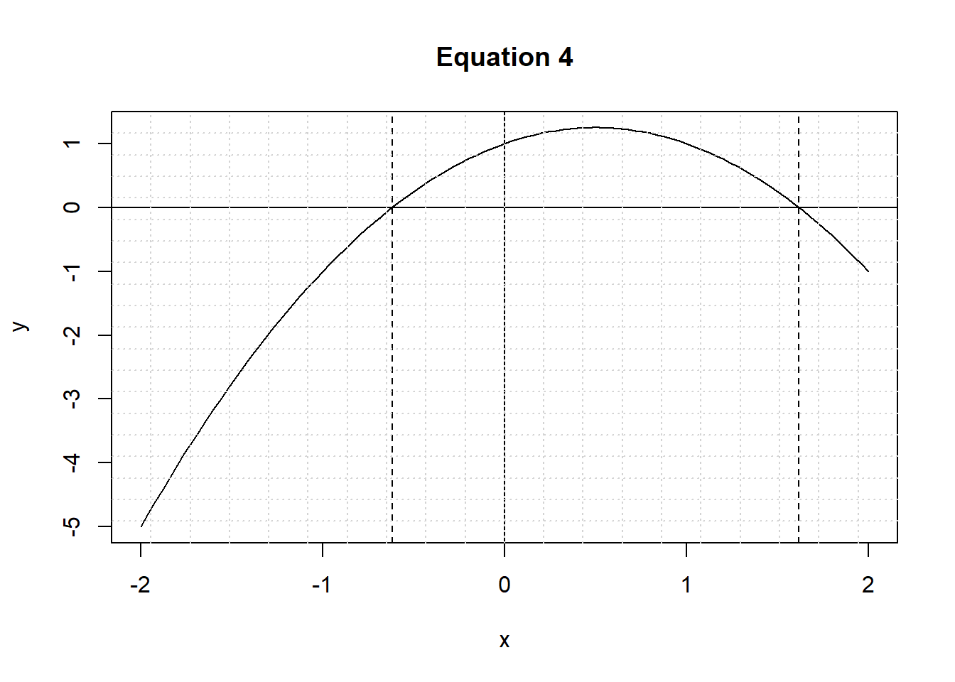
-x² + x = -1

# Solutions
(result(4,-20,25)) # Equation 1

## [1] 2.5

(result(1,20,19))  # Equation 2

## [1]  -1 -19

(result(-4,16,25)) # Equation 3

## [1] -1.201562  5.201562

curve(-4*x^2+16*x+25, from=-5, to=+8,xlab="x", ylab="y", main="Equation 3")
abline(h = 0, lty = 1)
abline(v = 0, lty = 1)
abline(v = -1.2016, lty = 2)
abline(v = +5.2016, lty = 2)
grid(nx = 50, ny = 50, col = "lightgray", lty = "dotted")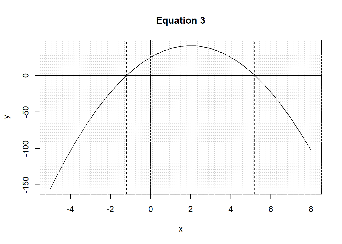

(result(-1,1,1)) # Equation 4

## [1] -0.618034  1.618034

curve(-1*x^2+1*x+1, from=-2, to=+2,xlab="x", ylab="y", main="Equation 4")
abline(h = 0, lty = 1)
abline(v = 0, lty = 1)
abline(v = -0.6180, lty = 2)
abline(v = +1.6180, lty = 2)
grid(nx = 20, ny = 20, col = "lightgray", lty = "dotted")