4 Random effects meta-analysis
4.1 A brief introduction to random effects models in meta-analysis
While fixed effects models are often thought of as the building blocks to meta-analysis, their strict assumptions (e.g., that all effect sizes come from the same underlying population) make them somewhat unrealistic starting points for ecological meta-analyses. As (Koricheva, Gurevitch, and Mengersen 2013) point out, we tend to use random effects models in ecological meta-analysis because even though the main effect we are investigating might be consistent across studies (e.g., changes in species richness) we want to also account for variation that comes from the individual studies that comprise our meta-analysis.
Random effects models account for the variation we get both within a study as well as between the many different studies in our meta-analysis.
Examples of random effects models in meta-analysis are plentiful, and researchers often begin with a random effects model, then progress onto more complex models that incorporate other variables from the data they’ve extracted. A study by (Murphy and Romanuk 2014) used a random effects model and aggregated over 300 effect sizes to find that in habitats with human disturbance, there was an average 18% decrease in species richness. In another meta-analysis, more focused on invasive species impacts, (Cameron, Vilà, and Cabeza 2016) brought together 112 articles and found that decomposition of leaf litter increased by 41% when invasive invertebrates were present in study sites.
4.2 Random effects model example
Just like in the previous chapter, we’ll use the example dataset for this book to walk through the steps involved in running and interpreting a random effects model in R. Then, we’ll plot the results in a forest plot.
First, we’ll load in the metafor package which we’ll use to run our models. Also, be sure that you have ggplot installed and loaded for one of the plots we’ll make in this chapter.
library(metafor)
library(ggplot2)
Next, be sure you have the dataframe RR_effect_sizes in your R environment (look for it in the environment tab of the top right panel if you are using Rstudio). You can always re-run the R code that is in chapters 1 and 2 of this book if the dataframe isn’t there.
The code below should look vaguely familiar from the last chapter on fixed-effects meta-analyses. That’s because we’re using the same function from metafor package called rma. Since we’ve already calculated an effect size for every pair of measurements in our database (i.e., invaded AND uninvaded richness) we’ll it in our modeling below. The column representing effect sizes is called yi in our dataframe, and each effect size has its own variance measure under the column vi.
random_effect_model_results <- rma(yi, # this is the effect size from each row in database
                                   vi, # measure of variance from each row in database
                                   method = "REML", # Using  a REML estimator which is common for random effect meta-analyses
                                   slab = paste(lastname, publication_year, sep = ""), # This line of code prepares study labels for the forest plot we'll create at the end of the chapter
                                   data = RR_effect_sizes) # Let R know the dataframe we'll use for our model calculations
## Warning: Studies with NAs omitted from model fitting.Because some measures of variation were listed as NA in our RR_effect_sizes dataframe, those entries will be dropped from our model.
Now, let’s look at the results of our random effects meta-analysis.
random_effect_model_results##
## Random-Effects Model (k = 84; tau^2 estimator: REML)
##
## tau^2 (estimated amount of total heterogeneity): 0.1720 (SE = 0.0327)
## tau (square root of estimated tau^2 value): 0.4147
## I^2 (total heterogeneity / total variability): 96.81%
## H^2 (total variability / sampling variability): 31.39
##
## Test for Heterogeneity:
## Q(df = 83) = 1034.0862, p-val < .0001
##
## Model Results:
##
## estimate se zval pval ci.lb ci.ub
## -0.2134 0.0509 -4.1948 <.0001 -0.3131 -0.1137 ***
##
## ---
## Signif. codes: 0 '***' 0.001 '**' 0.01 '*' 0.05 '.' 0.1 ' ' 1Initially, you’ll notice we get a few new metrics in this output when compared to the fixed-effects model. Let’s focus in on the output that’s relatively similar for now. Under the Model Results section you see that we get a summary effect size of -0.2134. Because the effect size is negative here, this indicates that we see an average decrease in species richness (the metric all of the articles in our meta-analysis measured) in invaded sites compared to control sites. This is a significant decrease in richness seeing that the p-value is <0.0001. We can also see the average decrease in richness is significant because the confidence interval produced by this random effects model does not include 0 (CI = -0.3131, -0.1137)
In order to see how the random effects model works a bit more clearly, we’ll use another function in the metafor package called rma.mv. The results from the rma function and this rma.mv will be the same. The difference is that when using rma.mv we have to indicate that we would like the model to account for random effects at the “effect size” level of our database.
This first line of code creates a new column in the RR_effect_sizes that assigns a unique number to every row in our database.
RR_effect_sizes$ID <- seq.int(nrow(RR_effect_sizes))Now, here’s the syntax for the rma.mv function. First, we specify the effect size column yi and the variance vi. Then we assign the random effect to every row in the database. Fortunately, we just created the ID variable which makes this easy using the syntax random = ~ 1 | ID. And lastly, we have to tell the function to pull all of these variables or columns from the dataframe RR_effect_sizes.
random_effect_model_results_again <- rma.mv(yi, vi, random = ~ 1 | ID, data = RR_effect_sizes)## Warning: Rows with NAs omitted from model fitting.random_effect_model_results_again##
## Multivariate Meta-Analysis Model (k = 84; method: REML)
##
## Variance Components:
##
## estim sqrt nlvls fixed factor
## sigma^2 0.1720 0.4147 84 no ID
##
## Test for Heterogeneity:
## Q(df = 83) = 1034.0862, p-val < .0001
##
## Model Results:
##
## estimate se zval pval ci.lb ci.ub
## -0.2134 0.0509 -4.1948 <.0001 -0.3131 -0.1137 ***
##
## ---
## Signif. codes: 0 '***' 0.001 '**' 0.01 '*' 0.05 '.' 0.1 ' ' 1When we print the results from the rma.mv function, we get the exact same results for the summary effect, p-value and confidence interval that we got from the rma function.
4.3 Accounting for nonindependence
However, because we don’t want the random effect model to assume that the random sources of variation are only coming from difference between the “trials” or the different rows in our database, we can instead assign the random effect to the lastname variable to account for the possibility that effect sizes are not completely independent (Cameron, Vilà, and Cabeza 2016). We do this because it is possible (and actually quite common) for meta-analysts to extract multiple effect sizes from the same article (i.e., the same article reports richness impacts of Zebra mussels and Quagga mussels separately).
random_effects_model_results_with_author <-
  rma.mv(yi,
         vi,
         random = ~ 1 | lastname,
         slab = paste(lastname, publication_year, sep = ""), # This line is important for when we create our forest plot later. It tells R that we want every row in our forst plot to have a label of author last name and the publication year.
         data = RR_effect_sizes)
## Warning: Rows with NAs omitted from model fitting.random_effects_model_results_with_author##
## Multivariate Meta-Analysis Model (k = 84; method: REML)
##
## Variance Components:
##
## estim sqrt nlvls fixed factor
## sigma^2 0.1096 0.3311 55 no lastname
##
## Test for Heterogeneity:
## Q(df = 83) = 1034.0862, p-val < .0001
##
## Model Results:
##
## estimate se zval pval ci.lb ci.ub
## -0.2368 0.0508 -4.6623 <.0001 -0.3363 -0.1373 ***
##
## ---
## Signif. codes: 0 '***' 0.001 '**' 0.01 '*' 0.05 '.' 0.1 ' ' 1Looking at the results from our updated random effects meta-analysis that controls for nonindependence, we see just slight shifts in these results. This is likely due to the relatively large sample size of our starting dataset. We now have an overall effect size of -0.2368, still suggesting a moderate decrease in richness when invasive species are present. We know this effect is significant because the p value is < 0.0001 and because the confidence interval does not overlap zero (CI = -0.3363, -0.1373.
4.4 Testing for heterogenity in your data
Cochran’s Q is a commonly used test for heterogeneity, and conveniently it’s part of the output from metafor’s random effect function. This statistic gives us the difference between each of the observed effect sizes in our dataset (so these are the yi’s and the effect size for a fixed effects model. While there’s a bit more detail to how we arrive at the Q statistic, ultimately those differences between the overall fixed effect size and each of our yi’s are squared so they won’t be negative and added up. One issue with Q statistic is that it always gets a higher magnitude when our sample size goes up.
Another way to explore potential publication bias in your datasets is by creating what are called publication bias histograms. To create publication bias histograms, you need to calculate all of individual (i.e., study-level) meta-analytic effect sizes. We already calculated these in chapter 2 with metafor’s escalc function.
For a reminder of what that dataframe looks like you can see:
datatable(RR_effect_sizes, fillContainer = TRUE)Then, we’ll create our histogram using the ggplot2 library. Set the x-axis as all of the different possible effect sizes in our dataset (in the table above they are labeled as yi) and the y-axis will show the count of each time the effect size appears in our dataset.
pub_bias_histogram <-ggplot(RR_effect_sizes, aes(x=yi)) +
   geom_histogram(binwidth=0.05,color="black", fill="white") +
   xlab("ln(Response ratio)") +
   ylab ("Frequency of effect sizes") +
   theme_cowplot() +
   theme(plot.title = element_text(size = 25, hjust = -.06, face = "bold"),
         axis.title = element_text(size = 25, face = "bold"),
         axis.text = element_text(size = 15)) +

   scale_y_continuous(expand = c(0,0),limits=c(0,10))
pub_bias_histogram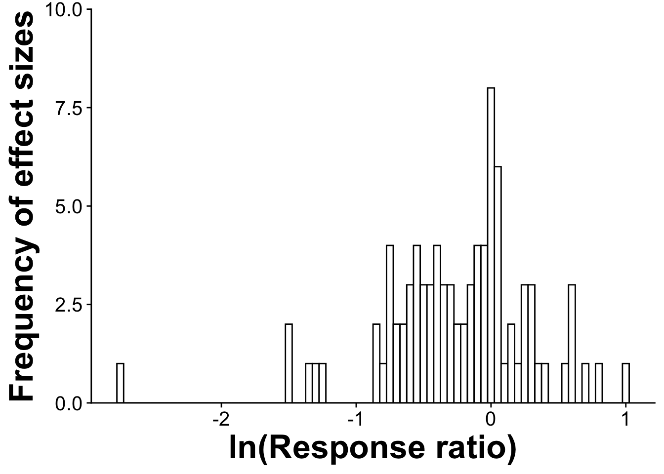
Figure 4.1: A publication bias histogram where relatively symmetrical histograms indicate a lack of publication bias in your dataset
For further information on use and to see examples of publication bias histograms in actions see (Crystal-Ornelas, Thapa, and Tully 2021; Thapa, Mirsky, and Tully 2018)
A last point to consider is that heterogeneity tests (in addition to the Q test there is the I^2 and tau-squared tests) they may be somewhat irrelevant since, by using a random effects model and acknowledging heterogeneity in our dataset by a priori choosing to use a random effects model over a fixed effects model to begin with (Koricheva, Gurevitch, and Mengersen 2013).
4.5 Forest plot for random effects model
Next, we’ll create a forest plot to visually display the results of our random effects meta-analytic model.
forest(
  RR_effect_sizes$yi, # These are effect sizes from each row in database
  RR_effect_sizes$vi, # These are variances from each row in database
  annotate = FALSE, # Setting this to false prevents R from including CIs for each of the 84 effect sizes in the forest plot. Setting it to TRUE is generally a good practice, but would make this plot cluttered.
  slab = random_effects_model_results_with_author$slab, # Along the left hand side, we want each individual effect size labeled with author names and publication years. We specified this when we calculated the summary effect size above
  xlab = "ln(Response Ratio)", # Label for x-axis
  cex = .8, # Text side for study labels
  pch = 15, # shape of bars in forest plot
  cex.lab = 1, # Size of x-axis label
)

# This is code adds in the summary effect size for your random effects meta-analysis
addpoly(
  random_effects_model_results_with_author, # specify the model where your summary effect comes from.
  col = "orange", # Pick a color that makes the summary effect stand out from the other effect sizes.
  cex = 1, # size for the text associates with summary effect
  annotate = TRUE, # Usually, we set this to true. It makes sure effect size and CI for summary effect size is printed on forest plot.
  mlab = "Summary" # Label for summary effect size
)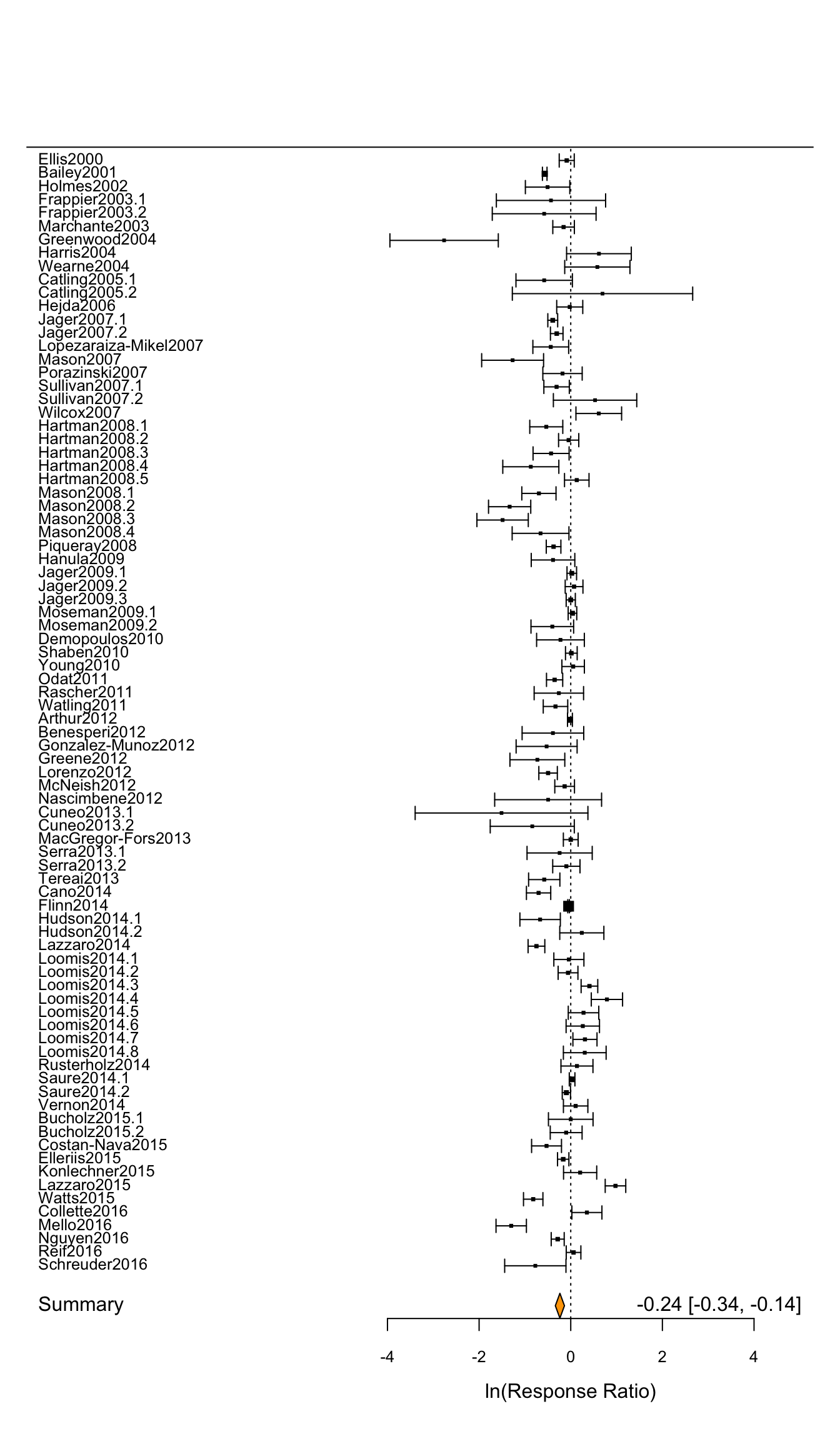
Figure 4.2: A forest plot displaying the results of our random effects meta-analysis
Just like in the previous chapter, this random effect forest plot shows all of the 84 individual effect sizes calculated in our meta-analysis (the horizontal black lines) as well as the summary statistic (the overall response ratio) for our random effects model that controls for non-independence that might come from effect sizes extracted from the same manuscript.
One thing that has changed in our random effects forest plot is that the results now reflect the results of our random effects model. So in the lower right hand corner of this figure we see the overall effect size of -0.2368 again suggesting a moderate decline in richness with the presence of invasive species. And we can tell this is a significant negative association because the orange diamond at the bottom of our forest plot does not overlap zero (CI = -0.3363, -0.1373.
Random effects models are helpful in accounting for the heterogeneity that is quite characteristic of studies in ecology, evolution, or the environmental sciences. With all of this heterogeneity you may want to see if there are some moderating variables within the dataset that drives the heterogeneity and explains some of the variation we see in our data. Methods for meta-regression will be explained in the next chapter.