Chapter 4 Assignment 3
Data Prep
url <- "https://www.dropbox.com/scl/fi/9ymxt900s77uq50ca6dgc/Enders-et-al.-2018-data.csv?rlkey=0rxjwleenhgu0gvzow5p0x9xf&dl=1"
df.aph <- read.csv(url)## EGA year long lat
## 1 0 2014 -95.16269 37.86238
## 2 0 2014 -95.28463 38.29669
## 3 0 2014 -95.33038 39.59482
## 4 0 2014 -95.32098 39.50696
## 5 0 2014 -98.55469 38.48455
## 6 0 2014 -98.84792 38.32772Data Exploration
# make SpatialPoints data frame
pts.sample <- data.frame(long = df.aph$long,lat = df.aph$lat,
                         count = df.aph$EGA,
                         t = df.aph$year)
coordinates(pts.sample) =~ long + lat
proj4string(pts.sample) <- CRS("+proj=longlat +datum=WGS84 +no_defs +ellps=WGS84 +towgs84=0,0,0")


# plot counts of EGA
par(mar=c(5.1, 4.1, 4.1, 8.1), xpd=TRUE)
plot(sf.kansas,main="Abundance of English Grain Aphid")
points(pts.sample[,1],col=rgb(0.4,0.8,0.5,0.9),pch=ifelse(pts.sample$count>0,20,4),cex=pts.sample$count/50+0.5)
legend("right",inset=c(-0.25,0),legend = c(0,1,10,20,40,60), bty = "n", text.col = "black",
       pch=c(4,20,20,20,20,20), cex=1.3,pt.cex=c(0,1,10,20,40,60)/50+0.5,col=rgb(0.4,0.8,0.5,0.9))
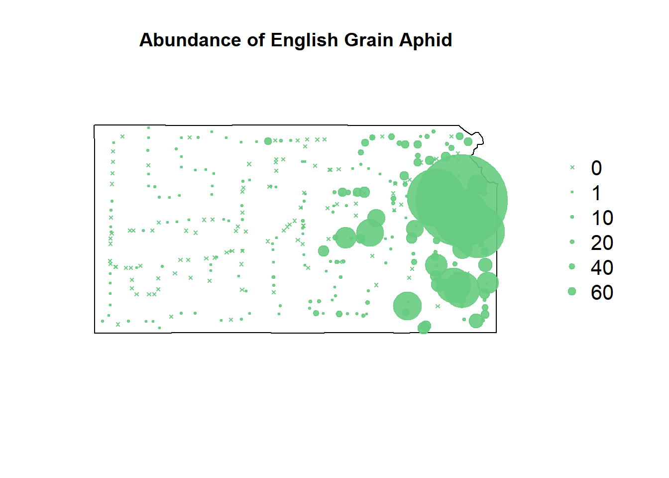
As a data scientist, I’m obsessed with over-fitting everything I can. I want two things with my models:
To fit a model that can plot the steep increase in EGA count seen near Kansas City
To determine if a different predictor variable can be used for EGA count
Looking at the NLCD website, it looks like cultivated crops fits a better definition of the vegetation I recall giving me ticks during summer concerts in that area, so I’ll fit the models to that variable as well.
Variable Prep
# using the img file is significantly faster than the url
# dear god
# https://www.dropbox.com/scl/fi/ew7yzm93aes7l8l37cn65/KS_2011_NLCD.img?rlkey=60ahyvxhq18gt0yr47tuq5fig&e=1&dl=0
rl.nlcd2011 <- raster("KS_2011_NLCD.img")
## Warning: Too large for int: nan (GDAL error 1)
## Warning: Too large for int: nan (GDAL error 1)## Warning: Too large for int: nan (GDAL error 1)
## Warning: Too large for int: nan (GDAL error 1)
## Warning: Too large for int: nan (GDAL error 1)
## Warning: Too large for int: nan (GDAL error 1)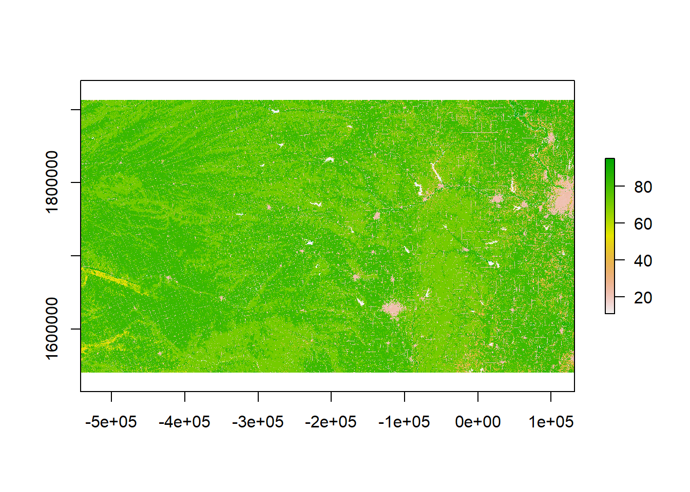
# original grassland variable selected for the formal study
rl.nlcd.grass <- rl.nlcd2011
rl.nlcd.grass[] <- ifelse(rl.nlcd.grass[]==71,1,0)
## Warning: Too large for int: nan (GDAL error 1)
## Warning: Too large for int: nan (GDAL error 1)
## Warning: Too large for int: nan (GDAL error 1)
## Warning: Too large for int: nan (GDAL error 1)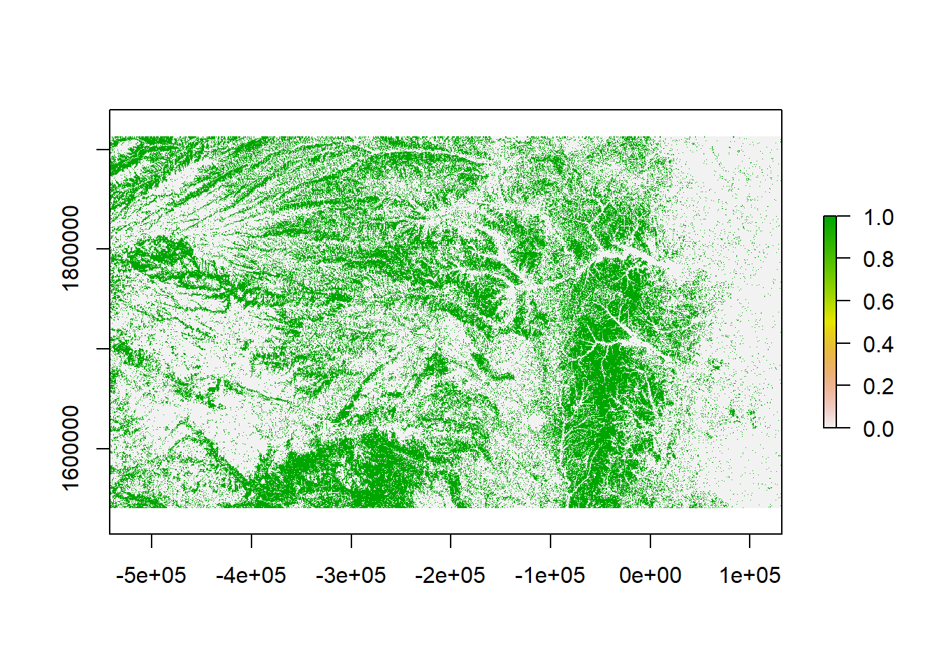
# raster of cultivated crops
rl.nlcd.cul <- rl.nlcd2011
rl.nlcd.cul[] <- ifelse(rl.nlcd.cul[]==82,1,0)
## Warning: Too large for int: nan (GDAL error 1)
## Warning: Too large for int: nan (GDAL error 1)
## Warning: Too large for int: nan (GDAL error 1)
## Warning: Too large for int: nan (GDAL error 1)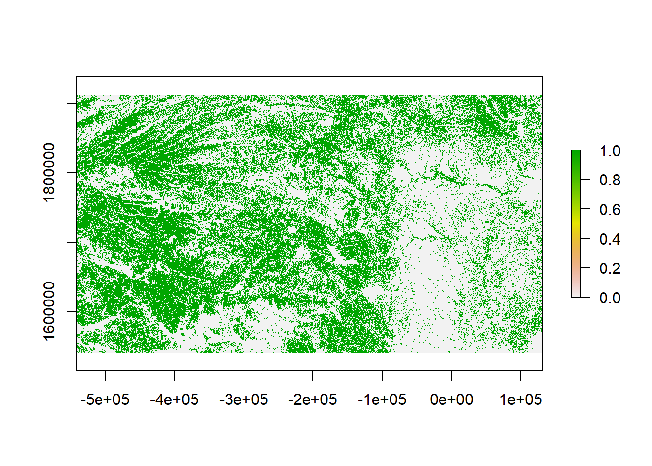
# calculate percentage of land area that is grassland
# within 5 km of sampled location
df.aph$grass.perc <- unlist(lapply(extract(rl.nlcd.grass,pts.sample,buffer=5000),mean))*100
## Warning in .local(x, y, ...): Transforming SpatialPoints to the crs of the
## Raster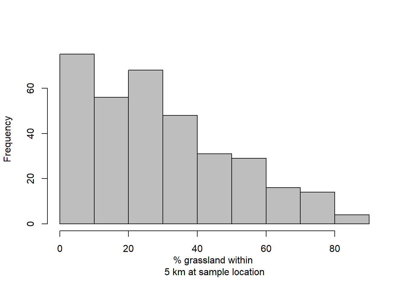
# calculate percentage of land area that is cultivated crops
# within 5 km of sampled location
df.aph$cul.perc <- unlist(lapply(extract(rl.nlcd.cul,pts.sample,buffer=5000),mean))*100
## Warning in .local(x, y, ...): Transforming SpatialPoints to the crs of the
## Raster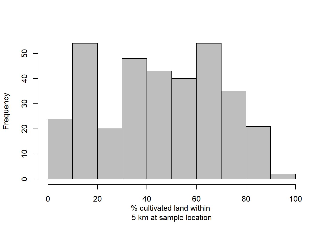
Grass Model Fitting
I’m using 4 “models”. Realistically, two of them are Poisson models fit to machine learning programs. gbm() allowing me to make use of the decision tree system (all models of decision trees suggest the creator of the convention hadn’t ever seen a tree) and rpart() will allow for the failure/deletion process for model paths with low predictive accuracy.
As with all machine learning programs there’s the concern of over-fitting and low forecasting efficacy.
The third model is a generalize linear model fit to a negative binomial, and the last model is the original zero-inflated Poisson that was presented in class. The last model will be used as a reference point for the capability of the other 3 models.
# model fitting based on grass percentage

set.seed(73)

# poisson distributed gbm
m1 <- gbm(EGA ~ grass.perc + as.factor(year) + df.aph$long + df.aph$lat, data=df.aph, distribution="poisson")

# poisson distributed rpart
m2 <- rpart(EGA ~ grass.perc + as.factor(year) + df.aph$long + df.aph$lat,data=df.aph,method="poisson",control=rpart.control(cp = 0.0001))

# negative binomial
m3 <- glm.nb(EGA ~ grass.perc + as.factor(year) + df.aph$long + df.aph$lat, data=df.aph)

# hefley zip model for comparison
m4 <- gam(list(EGA ~ grass.perc + as.factor(year) + s(long,lat, bs = "gp"), ~ grass.perc),
          family = ziplss(), data = df.aph)
Grass Model Checking
As any good programmer does, I’ve poached a significant amount of my code from someone who already suffered for it. I’ll be using a few of the original model checks from the example for models 3 and 4.
Concurvity and variogram have been left out as checks for two reasons:
I have one
gam()functionThey broke the bookdown horrendously
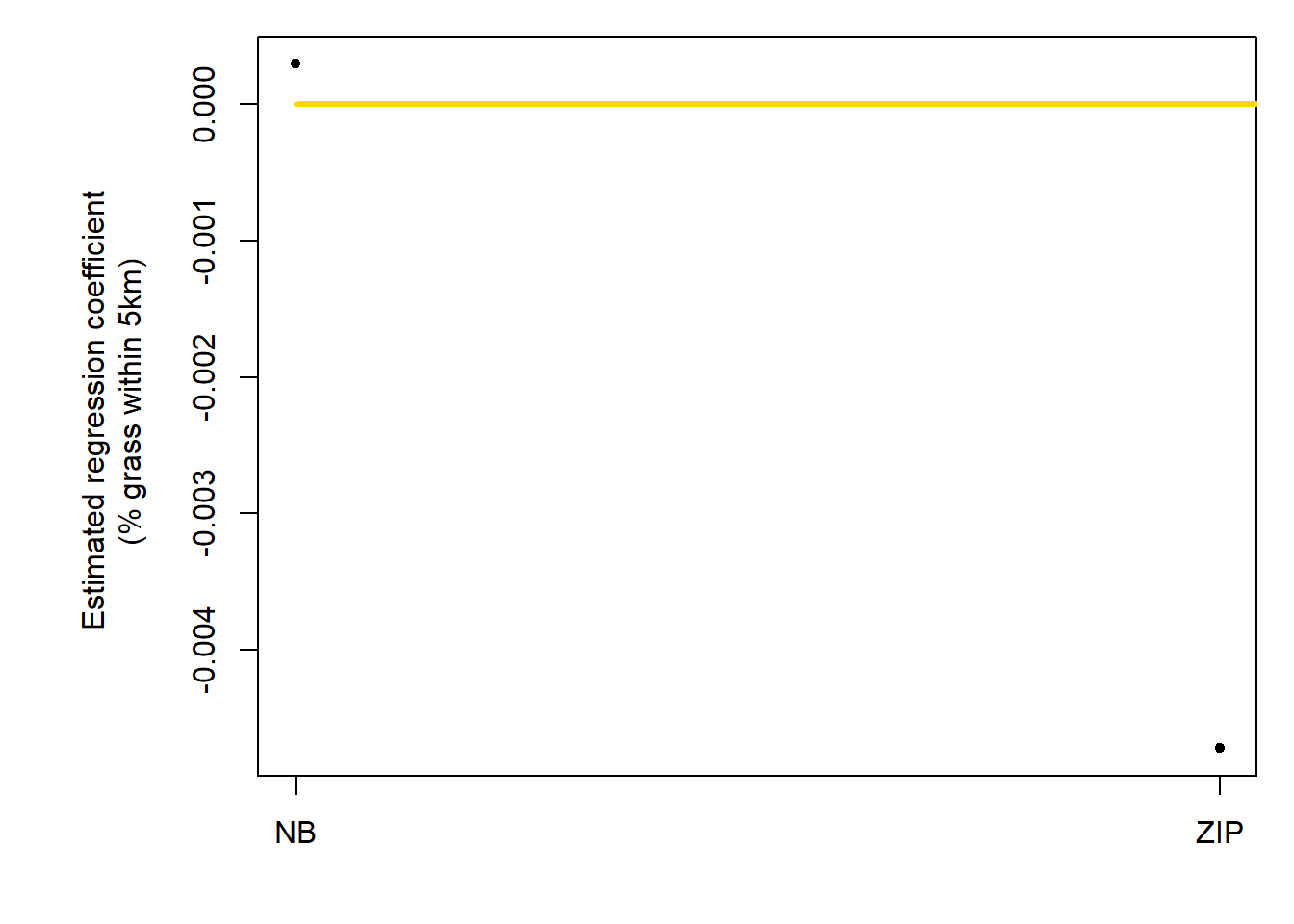
# regression coefficients
b1.hat <- c(coef(m3)[2],coef(m4)[2])

b1.hat.m <- c("Negative Binomial",
            "Zero-Inflated Poisson")
all.models <- str_wrap(b1.hat.m, width = 15)
grass.perc <- b1.hat
b1.hat.tab <- data.frame(all.models, grass.perc)
b1.hat.tab
## all.models grass.perc
## 1 Negative\nBinomial -0.002891876
## 2 Zero-Inflated\nPoisson -0.009865298# Abundance at 0% grassland/Abundance at 100% grassland
zero.abund <- exp(b1.hat[1:2]*0)/exp(b1.hat[1:2]*100)
b1.hat.tab <- data.frame(all.models, grass.perc, zero.abund)
b1.hat.tab## all.models grass.perc zero.abund
## 1 Negative\nBinomial -0.002891876 1.335342
## 2 Zero-Inflated\nPoisson -0.009865298 2.681912ucl <- c(confint.default(m3,parm="grass.perc")[2],confint.default(m4,parm="grass.perc")[2])
lcl <- c(confint.default(m3,parm="grass.perc")[1],confint.default(m4,parm="grass.perc")[1])
par(mar=c(4,7,1,1))
plotCI(c(1:2), b1.hat, ui=ucl, li=lcl,pch=20,xaxt="n",xlab="",ylab="Estimated regression coefficient \n (% grass within 5km)")
lines(c(1,3),c(0,0),col="gold",lwd=3)
axis(at=c(1:2),lab=c("NB","ZIP"),side=1)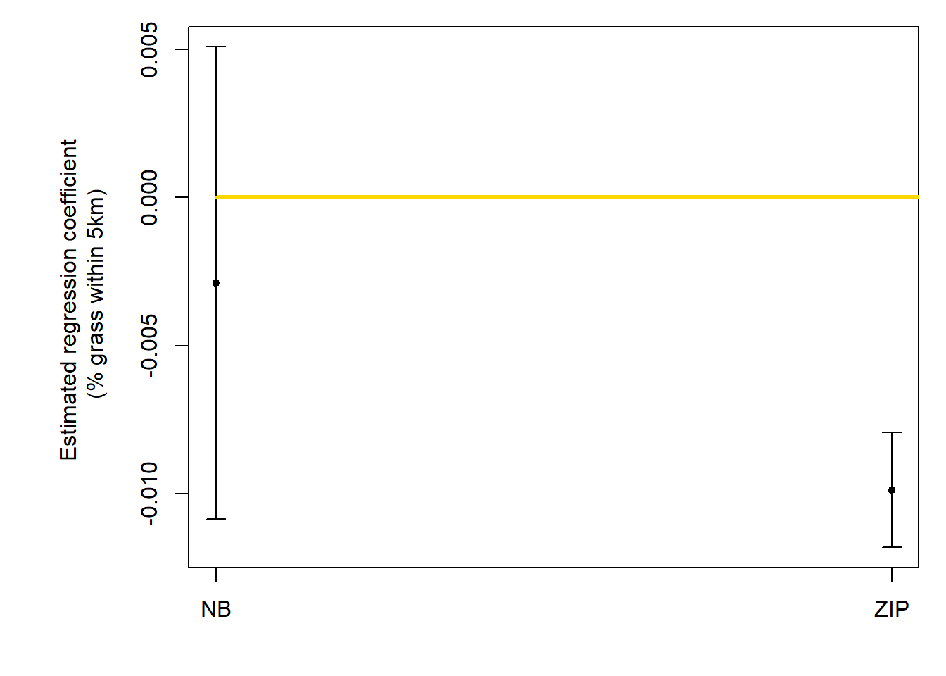
## grass.perc.1
## 0.0005674407## 2.5 % 97.5 %
## grass.perc.1 -0.006196991 0.007331872## (Intercept).1
## NA## (Intercept).1
## NA## df AIC
## m3 6.00000 1927.335
## m4 36.73709 10496.127It’s hard enough to make inferences off of these metrics since I don’t have immense experience with them, but the zero-inflated model performing better isn’t hard to see.
The real problem is that model checking isn’t consistent across all 4 of the models being used, since machine learning models either:
Lack the same model checks outright
Have them placed somewhere so un-intuitive that documentation couldn’t rescue me this time
# Compare expected number of zeros to observed
# Observed number of zeros
length(which(df.aph$EGA == 0))## [1] 125# Expected number of sites with zero counts under m1 (Poisson distribution)
mu <- predict(m1, type="response", newdata=df.aph)## Using 100 trees...## [1] 7.412335# Expected number of sites with zero counts under m2 (Poisson distribution)
mu <- predict(m2, type="vector", newdata=df.aph)
sum(exp(-mu))## [1] 95.46695# Expected number of sites with zero counts under m3 (Negative binomial distribution)
mu <- predict(m3, type="response", newdata=df.aph)
sum(exp(-mu))## [1] 87.26908# Expected number of sites with zero counts under m4 (Zero inflated Poisson)
mu <- exp(predict(m4)[,1])
p <- 1/(1+exp(-predict(m4)[,2]))
sum(p*exp(-mu) + (1-p))## [1] 215.5657From the perspective of predicting zeros, the zero-inflated Poisson is significantly better than the rest. The gradient boosted Poisson is actually awful at predicting zeros, and my guess would be that it smoothed out all of the data across every available point. While this makes a lot of sense for something like a spatial heat map, it’s pretty terrible for deciding if we should or should not go sample an area.
One could argue that it’s possible the scientists performing the sampling were more prone to error in their sampling than they were in their selection process for areas of Kansas, but that would only make sense if their sole sampling goal was EGA.
Graphical diagnostics are my preference, they’re comfortable and tell me a lot more about what’s going on with my models than regression diagnostics (for now). As it was pointed out in class, stick with what you know and get an outside consult.
Grass Graphics
Working title was “Grassphics”.
I’ll save discussion on these for the end, since there’s so many of them.
# gbm predictions
df.pred.tmp <- data.frame(EGA = NA,
year = df.aph$year,
long = df.aph$long,
lat = df.aph$lat,
grass.perc = df.aph$grass.perc,
cul.perc = df.aph$cul.perc)
df.pred.tmp$EGA <- predict.gbm(m1, newdata=df.pred.tmp, type="response")## Using 100 trees...# reformat predictions for shapefile plotting
pts.sample <- data.frame(long = df.aph$long,lat = df.aph$lat,
count = df.pred.tmp$EGA,
t = df.aph$year)
coordinates(pts.sample) =~ long + lat
proj4string(pts.sample) <- CRS("+proj=longlat +datum=WGS84 +no_defs +ellps=WGS84 +towgs84=0,0,0")
# plot expected counts of EGA
par(mar=c(5.1, 4.1, 4.1, 8.1), xpd=TRUE)
plot(sf.kansas,main="Expected Abundance of English Grain Aphid")
points(pts.sample[,1],col=rgb(0.4,0.8,0.5,0.9),pch=ifelse(pts.sample$count>0,20,4),cex=pts.sample$count/50+0.5)
legend("right",inset=c(-0.25,0),legend = c(0,1,10,20,40,60), bty = "n", text.col = "black",
pch=c(4,20,20,20,20,20), cex=1.3,pt.cex=c(0,1,10,20,40,60)/50+0.5,col=rgb(0.4,0.8,0.5,0.9))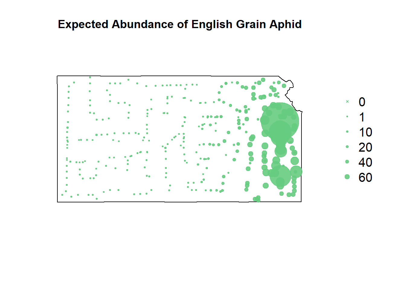
# rpart predictions
df.pred.tmp <- data.frame(EGA = NA,
year = df.aph$year,
long = df.aph$long,
lat = df.aph$lat,
grass.perc = df.aph$grass.perc,
cul.perc = df.aph$cul.perc)
df.pred.tmp$EGA <- predict(m2, newdata=df.pred.tmp, type="vector")
# reformat predictions for shapefile plotting
pts.sample <- data.frame(long = df.aph$long,lat = df.aph$lat,
count = df.pred.tmp$EGA,
t = df.aph$year)
coordinates(pts.sample) =~ long + lat
proj4string(pts.sample) <- CRS("+proj=longlat +datum=WGS84 +no_defs +ellps=WGS84 +towgs84=0,0,0")
# plot expected counts of EGA
par(mar=c(5.1, 4.1, 4.1, 8.1), xpd=TRUE)
plot(sf.kansas,main="Expected Abundance of English Grain Aphid")
points(pts.sample[,1],col=rgb(0.4,0.8,0.5,0.9),pch=ifelse(pts.sample$count>0,20,4),cex=pts.sample$count/50+0.5)
legend("right",inset=c(-0.25,0),legend = c(0,1,10,20,40,60), bty = "n", text.col = "black",
pch=c(4,20,20,20,20,20), cex=1.3,pt.cex=c(0,1,10,20,40,60)/50+0.5,col=rgb(0.4,0.8,0.5,0.9))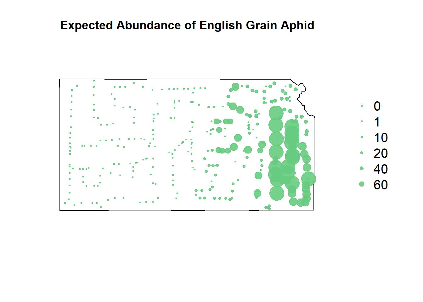
# negative binomial predictions
df.pred.tmp <- data.frame(EGA = NA,
year = df.aph$year,
long = df.aph$long,
lat = df.aph$lat,
grass.perc = df.aph$grass.perc,
cul.perc = df.aph$cul.perc)
df.pred.tmp$EGA <- predict(m3, newdata=df.pred.tmp, type="response")
# reformat predictions for shapefile plotting
pts.sample <- data.frame(long = df.aph$long,lat = df.aph$lat,
count = df.pred.tmp$EGA,
t = df.aph$year)
coordinates(pts.sample) =~ long + lat
proj4string(pts.sample) <- CRS("+proj=longlat +datum=WGS84 +no_defs +ellps=WGS84 +towgs84=0,0,0")
# plot expected counts of EGA
par(mar=c(5.1, 4.1, 4.1, 8.1), xpd=TRUE)
plot(sf.kansas,main="Expected Abundance of English Grain Aphid")
points(pts.sample[,1],col=rgb(0.4,0.8,0.5,0.9),pch=ifelse(pts.sample$count>0,20,4),cex=pts.sample$count/50+0.5)
legend("right",inset=c(-0.25,0),legend = c(0,1,10,20,40,60), bty = "n", text.col = "black",
pch=c(4,20,20,20,20,20), cex=1.3,pt.cex=c(0,1,10,20,40,60)/50+0.5,col=rgb(0.4,0.8,0.5,0.9))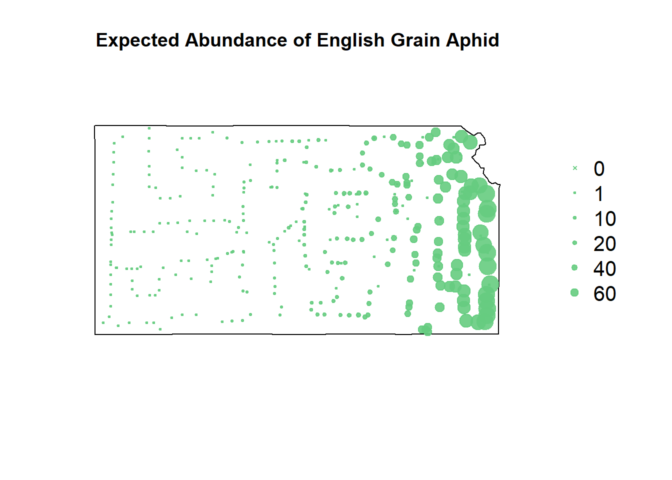
# zip predictions
df.pred.tmp <- data.frame(EGA = NA,
year = df.aph$year,
long = df.aph$long,
lat = df.aph$lat,
grass.perc = df.aph$grass.perc,
cul.perc = df.aph$cul.perc)
df.pred.tmp$EGA <- predict(m4, newdata=df.pred.tmp, type="response")
# reformat predictions for shapefile plotting
pts.sample <- data.frame(long = df.aph$long,lat = df.aph$lat,
count = df.pred.tmp$EGA,
t = df.aph$year)
coordinates(pts.sample) =~ long + lat
proj4string(pts.sample) <- CRS("+proj=longlat +datum=WGS84 +no_defs +ellps=WGS84 +towgs84=0,0,0")
# plot expected counts of EGA
par(mar=c(5.1, 4.1, 4.1, 8.1), xpd=TRUE)
plot(sf.kansas,main="Expected Abundance of English Grain Aphid")
points(pts.sample[,1],col=rgb(0.4,0.8,0.5,0.9),pch=ifelse(pts.sample$count>0,20,4),cex=pts.sample$count/50+0.5)
legend("right",inset=c(-0.25,0),legend = c(0,1,10,20,40,60), bty = "n", text.col = "black",
pch=c(4,20,20,20,20,20), cex=1.3,pt.cex=c(0,1,10,20,40,60)/50+0.5,col=rgb(0.4,0.8,0.5,0.9))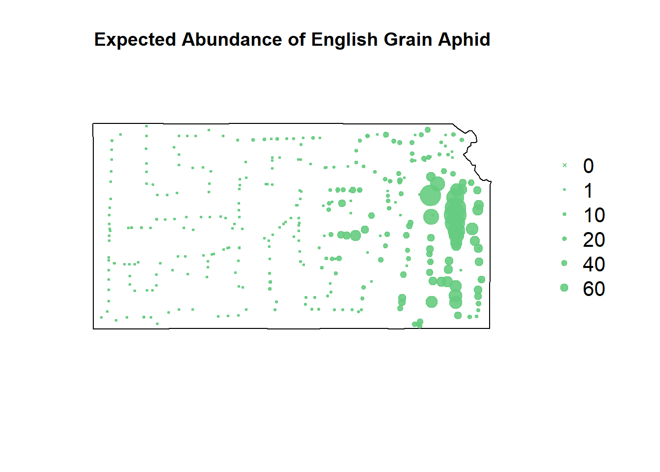
# rebuild original count visualization
{
# make SpatialPoints data frame
pts.sample <- data.frame(long = df.aph$long,lat = df.aph$lat,
count = df.aph$EGA,
t = df.aph$year)
coordinates(pts.sample) =~ long + lat
proj4string(pts.sample) <- CRS("+proj=longlat +datum=WGS84 +no_defs +ellps=WGS84 +towgs84=0,0,0")
# plot counts of EGA
par(mar=c(5.1, 4.1, 4.1, 8.1), xpd=TRUE)
plot(sf.kansas,main="Abundance of English Grain Aphid")
points(pts.sample[,1],col=rgb(0.4,0.8,0.5,0.9),pch=ifelse(pts.sample$count>0,20,4),cex=pts.sample$count/50+0.5)
legend("right",inset=c(-0.25,0),legend = c(0,1,10,20,40,60), bty = "n", text.col = "black",
pch=c(4,20,20,20,20,20), cex=1.3,pt.cex=c(0,1,10,20,40,60)/50+0.5,col=rgb(0.4,0.8,0.5,0.9))
}
Despite the gradient-boosted model being awful at predicting where the EGA counts won’t occur, it’s fit well to the upticks in their counts.
Recursive partitioning smooths things out a lot more, making more of a heat map of where to focus our sampling rather than telling us where we’ll get highest sampling value.
The negative binomial model somehow takes the negatives of both the gradient-boosted and the recursive partitioning models and smashes them together.
The zero-inflated model seemingly smooths everything out, but it’s ability to predict zero counts can’t be denied.
Crop Model Fitting
Now I’ll fit the exact same 4 models with the replacement of cultivated crops for the grassland variable.
# model fitting based on cultivated crop percentage
# poisson distributed gbm
m1 <- gbm(EGA ~ cul.perc + as.factor(year) + df.aph$long + df.aph$lat, data=df.aph, distribution="poisson")
# poisson distributed rpart
m2 <- rpart(EGA ~ cul.perc + as.factor(year) + df.aph$long + df.aph$lat,data=df.aph,method="poisson",control=rpart.control(cp = 0.0001))
# negative binomial
m3 <- glm.nb(EGA ~ cul.perc + as.factor(year) + df.aph$long + df.aph$lat, data=df.aph)
# hefley ziplss model for comparison
m4 <- gam(list(EGA ~ cul.perc + as.factor(year) + s(long,lat, bs = "gp"), ~ cul.perc),
family = ziplss(), data = df.aph)Crop Model Checking
# model 3 and 4 checks again
{
# regression coefficients
b1.hat <- c(coef(m3)[2],coef(m4)[2])
b1.hat.m <- c("Negative Binomial",
"Zero-Inflated Poisson")
all.models <- str_wrap(b1.hat.m, width = 15)
grass.perc <- b1.hat
b1.hat.tab <- data.frame(all.models, grass.perc)
b1.hat.tab
# Abundance at 0% grassland/Abundance at 100% grassland
zero.abund <- exp(b1.hat[1:2]*0)/exp(b1.hat[1:2]*100)
b1.hat.tab <- data.frame(all.models, grass.perc, zero.abund)
b1.hat.tab
ucl <- c(confint.default(m3,parm="grass.perc")[2],confint.default(m4,parm="grass.perc")[2])
lcl <- c(confint.default(m3,parm="grass.perc")[1],confint.default(m4,parm="grass.perc")[1])

par(mar=c(4,7,1,1))
plotCI(c(1:2), b1.hat, ui=ucl, li=lcl,pch=20,xaxt="n",xlab="",ylab="Estimated regression coefficient \n (% grass within 5km)")
lines(c(1,3),c(0,0),col="gold",lwd=3)
axis(at=c(1:2),lab=c("NB","ZIP"),side=1)
# Examing regression coefficients for zero-inflated portion of model 4
coef(m3)[37]
confint.default(m3,parm="grass.perc.1")
# Probability of zero inflation at 0% grassland
1 - 1/(1+exp(-(coef(m3)[36]+coef(m3)[37]*0)))
# Probability of zero inflation at 100% grassland
1 - 1/(1+exp(-(coef(m3)[36]+coef(m3)[37]*100)))
# Compare models using AIC (see pgs. 284-286 in Wikle et al. 2019)
AIC(m3,m4)
}
## df AIC
## m3 6.0000 1927.747
## m4 36.7715 10571.743Models 3 and 4 present as being marginally worse with this predictor variable.
# Compare expected number of zeros to observed
# Observed number of zeros
length(which(df.aph$EGA == 0))
## [1] 125# Expected number of sites with zero counts under m1 (Poisson distribution)
mu <- predict(m1, type="response", newdata=df.aph)## Using 100 trees...## [1] 7.300712# Expected number of sites with zero counts under m2 (Poisson distribution)
mu <- predict(m2, type="vector", newdata=df.aph)
sum(exp(-mu))## [1] 97.1132# Expected number of sites with zero counts under m3 (Negative binomial distribution)
mu <- predict(m3, type="response", newdata=df.aph)
sum(exp(-mu))## [1] 87.87259# Expected number of sites with zero counts under m4 (Zero inflated Poisson)
mu <- exp(predict(m4)[,1])
p <- 1/(1+exp(-predict(m4)[,2]))
sum(p*exp(-mu) + (1-p))## [1] 213.3464On regression diagnostics alone, these models are all slightly more terrible at making predictions.
Again, I feel more confident making inferences off of graphics.
Crop Graphics
The working title wasn’t very academic.
Discussion is left for the end again.
# gbm predictions
df.pred.tmp <- data.frame(EGA = NA,
                          year = df.aph$year,
                          long = df.aph$long,
                          lat = df.aph$lat,
                          grass.perc = df.aph$grass.perc,
                          cul.perc = df.aph$cul.perc)

df.pred.tmp$EGA <- predict.gbm(m1, newdata=df.pred.tmp, type="response")
## Using 100 trees...# reformat predictions for shapefile plotting
pts.sample <- data.frame(long = df.aph$long,lat = df.aph$lat,
count = df.pred.tmp$EGA,
t = df.aph$year)
coordinates(pts.sample) =~ long + lat
proj4string(pts.sample) <- CRS("+proj=longlat +datum=WGS84 +no_defs +ellps=WGS84 +towgs84=0,0,0")
# plot expected counts of EGA
par(mar=c(5.1, 4.1, 4.1, 8.1), xpd=TRUE)
plot(sf.kansas,main="Expected Abundance of English Grain Aphid")
points(pts.sample[,1],col=rgb(0.4,0.8,0.5,0.9),pch=ifelse(pts.sample$count>0,20,4),cex=pts.sample$count/50+0.5)
legend("right",inset=c(-0.25,0),legend = c(0,1,10,20,40,60), bty = "n", text.col = "black",
pch=c(4,20,20,20,20,20), cex=1.3,pt.cex=c(0,1,10,20,40,60)/50+0.5,col=rgb(0.4,0.8,0.5,0.9))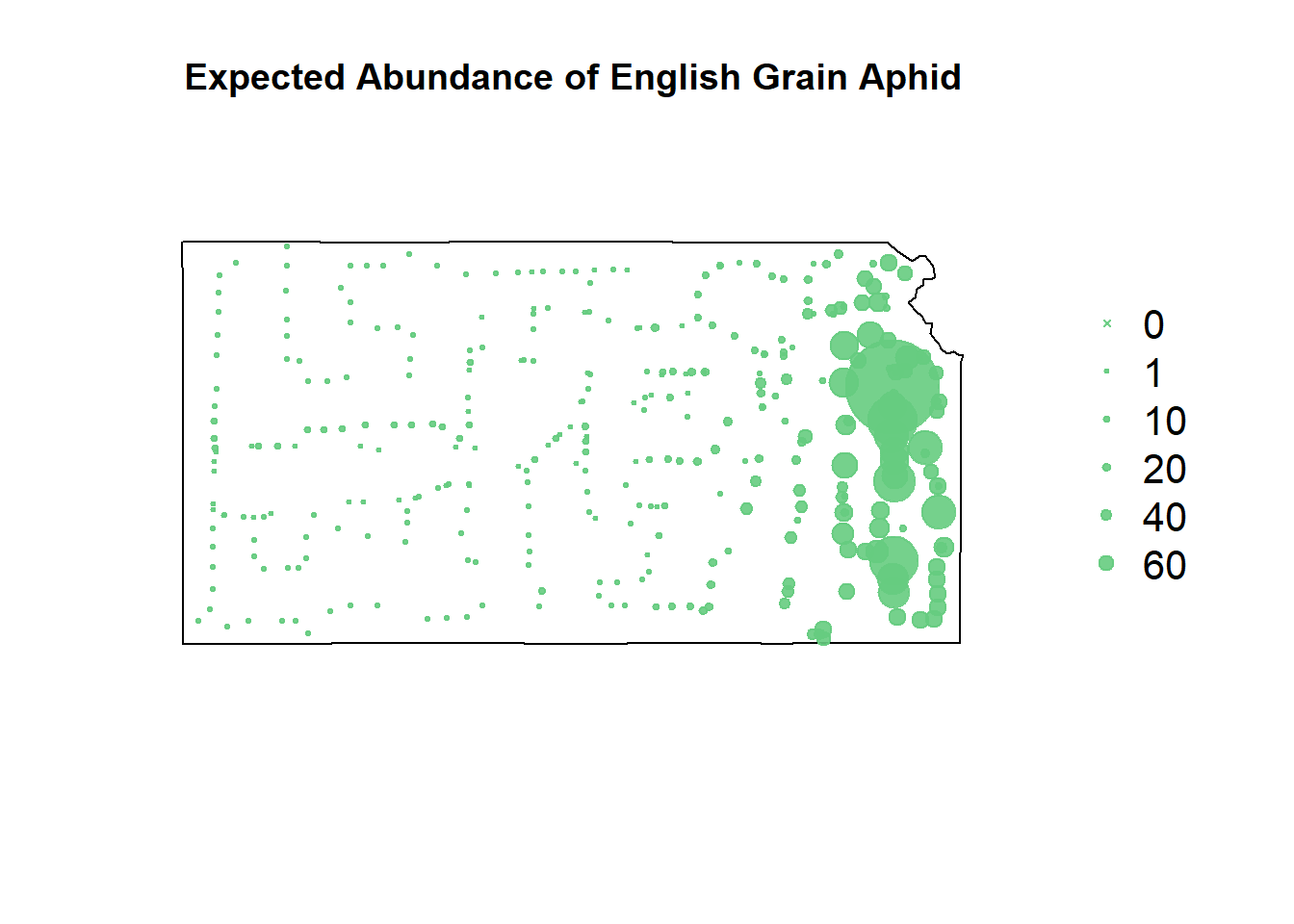
# rpart predictions
df.pred.tmp <- data.frame(EGA = NA,
year = df.aph$year,
long = df.aph$long,
lat = df.aph$lat,
grass.perc = df.aph$grass.perc,
cul.perc = df.aph$cul.perc)
df.pred.tmp$EGA <- predict(m2, newdata=df.pred.tmp, type="vector")
# reformat predictions for shapefile plotting
pts.sample <- data.frame(long = df.aph$long,lat = df.aph$lat,
                         count = df.pred.tmp$EGA,
                         t = df.aph$year)
coordinates(pts.sample) =~ long + lat
proj4string(pts.sample) <- CRS("+proj=longlat +datum=WGS84 +no_defs +ellps=WGS84 +towgs84=0,0,0")

# plot expected counts of EGA
par(mar=c(5.1, 4.1, 4.1, 8.1), xpd=TRUE)
plot(sf.kansas,main="Expected Abundance of English Grain Aphid")
points(pts.sample[,1],col=rgb(0.4,0.8,0.5,0.9),pch=ifelse(pts.sample$count>0,20,4),cex=pts.sample$count/50+0.5)
legend("right",inset=c(-0.25,0),legend = c(0,1,10,20,40,60), bty = "n", text.col = "black",
       pch=c(4,20,20,20,20,20), cex=1.3,pt.cex=c(0,1,10,20,40,60)/50+0.5,col=rgb(0.4,0.8,0.5,0.9))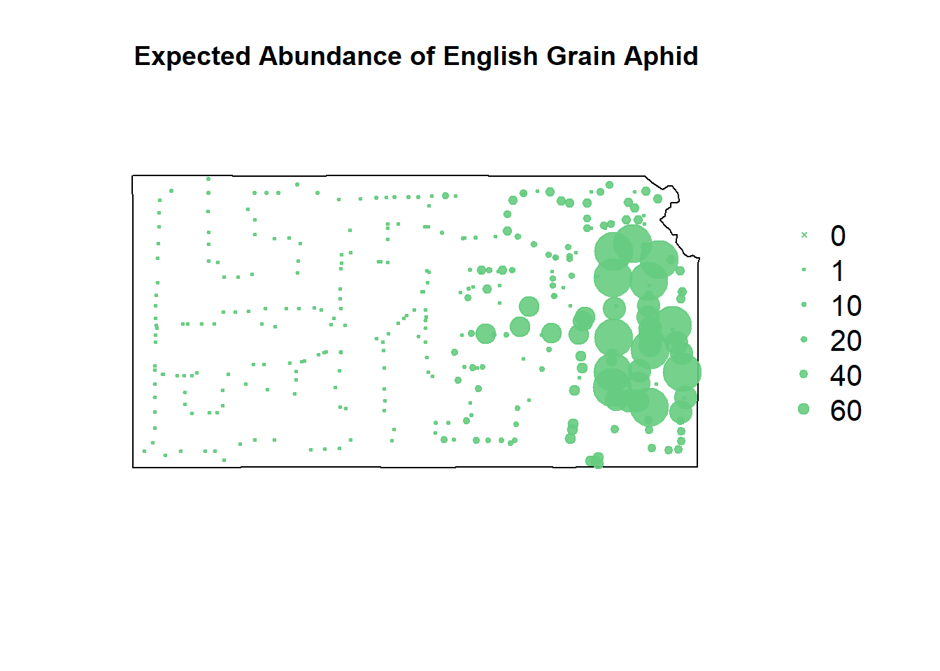
# negative binomial predictions
df.pred.tmp <- data.frame(EGA = NA,
                          year = df.aph$year,
                          long = df.aph$long,
                          lat = df.aph$lat,
                          grass.perc = df.aph$grass.perc,
                          cul.perc = df.aph$cul.perc)

df.pred.tmp$EGA <- predict(m3, newdata=df.pred.tmp, type="response")

# reformat predictions for shapefile plotting
pts.sample <- data.frame(long = df.aph$long,lat = df.aph$lat,
                         count = df.pred.tmp$EGA,
                         t = df.aph$year)
coordinates(pts.sample) =~ long + lat
proj4string(pts.sample) <- CRS("+proj=longlat +datum=WGS84 +no_defs +ellps=WGS84 +towgs84=0,0,0")

# plot expected counts of EGA
par(mar=c(5.1, 4.1, 4.1, 8.1), xpd=TRUE)
plot(sf.kansas,main="Expected Abundance of English Grain Aphid")
points(pts.sample[,1],col=rgb(0.4,0.8,0.5,0.9),pch=ifelse(pts.sample$count>0,20,4),cex=pts.sample$count/50+0.5)
legend("right",inset=c(-0.25,0),legend = c(0,1,10,20,40,60), bty = "n", text.col = "black",
       pch=c(4,20,20,20,20,20), cex=1.3,pt.cex=c(0,1,10,20,40,60)/50+0.5,col=rgb(0.4,0.8,0.5,0.9))
# zip predictions
df.pred.tmp <- data.frame(EGA = NA,
                          year = df.aph$year,
                          long = df.aph$long,
                          lat = df.aph$lat,
                          grass.perc = df.aph$grass.perc,
                          cul.perc = df.aph$cul.perc)

df.pred.tmp$EGA <- predict(m4, newdata=df.pred.tmp, type="response")

# reformat predictions for shapefile plotting
pts.sample <- data.frame(long = df.aph$long,lat = df.aph$lat,
                         count = df.pred.tmp$EGA,
                         t = df.aph$year)
coordinates(pts.sample) =~ long + lat
proj4string(pts.sample) <- CRS("+proj=longlat +datum=WGS84 +no_defs +ellps=WGS84 +towgs84=0,0,0")

# plot expected counts of EGA
par(mar=c(5.1, 4.1, 4.1, 8.1), xpd=TRUE)
plot(sf.kansas,main="Expected Abundance of English Grain Aphid")
points(pts.sample[,1],col=rgb(0.4,0.8,0.5,0.9),pch=ifelse(pts.sample$count>0,20,4),cex=pts.sample$count/50+0.5)
legend("right",inset=c(-0.25,0),legend = c(0,1,10,20,40,60), bty = "n", text.col = "black",
       pch=c(4,20,20,20,20,20), cex=1.3,pt.cex=c(0,1,10,20,40,60)/50+0.5,col=rgb(0.4,0.8,0.5,0.9))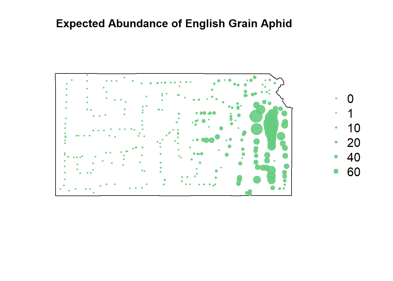
# rebuild original count visualization
{
  # make SpatialPoints data frame
  pts.sample <- data.frame(long = df.aph$long,lat = df.aph$lat,
                           count = df.aph$EGA,
                           t = df.aph$year)
  coordinates(pts.sample) =~ long + lat
  proj4string(pts.sample) <- CRS("+proj=longlat +datum=WGS84 +no_defs +ellps=WGS84 +towgs84=0,0,0")


  # plot counts of EGA
  par(mar=c(5.1, 4.1, 4.1, 8.1), xpd=TRUE)
  plot(sf.kansas,main="Abundance of English Grain Aphid")
  points(pts.sample[,1],col=rgb(0.4,0.8,0.5,0.9),pch=ifelse(pts.sample$count>0,20,4),cex=pts.sample$count/50+0.5)
  legend("right",inset=c(-0.25,0),legend = c(0,1,10,20,40,60), bty = "n", text.col = "black",
         pch=c(4,20,20,20,20,20), cex=1.3,pt.cex=c(0,1,10,20,40,60)/50+0.5,col=rgb(0.4,0.8,0.5,0.9))
}
Cultivated crops is just not a good predictor variable. There’s not much elegant wording that can be used here.
It was believable that crops would attract the aphids, but more believable that they’d be indiscriminate. Wheat/Grain is likely just an analog to their natural habitat. Its also very likely I misunderstood the NLCD website legend.
Overall, the models are doing the exact same things they were doing before. They’re just doing it a lot worse.
Closing Discussion
When everything is stacked up, a single theme is clear.
Statistical models are only as good as the task they’re being asked to perform.
The zero-inflated model is excellent as telling us where the aphids will and won’t be, but it’s not good at telling us how many there will be.
The two machine learning models had wildly different results, which actually makes sense to their different methodologies.
Gradient-boosting uses decision trees, it’s goal is to try to achieve results through yes/no (or) if/else logic. As the trees advance they’re minimizing error rather than an arbitrary failure condition.
Recursive partitioning works closer to what we see with current generative AI. It’s a more or less a primitive version of the “cake” system that things like OpenAI software use. When a split off of the model hits a certain failure condition it’s destroyed, and only the most successful splits are retained.
The negative binomial ended up being the most reliable calibrator for failure. It didn’t achieve much beyond missing the bar for everything it could possibly try to be good at.
Grassland is the better predictor variable to make use of, which makes sense considering the source material was published a while ago and it’s easy to believe the original authors would have spent a lot more time on the predictors than my general curiosity could achieve.
If anything, the major output of inspecting cultivated crops as a variable revealed three things:
The NCLD legend is mildly vague on it’s descriptions
EGA likely don’t differentiate between wild grains and cultivated grains
I’m not sure which wheat field near Kansas City I was in last summer