Chapter 2 Assignment 1
Data Prep
Package explanations:
sf: GIS work in R
lubridate: manipulating date/time data
mgcv: contains the
gam()function (generalized additive model)gbm: contains the
gbm()function (gradient boosted regression ML)
The raw data from the Strava phone app, (GPS tracking, used for running), followed by the cleaning and conversion of the data into .kml:
url <- "https://www.dropbox.com/scl/fi/p5166cbqhof62a916r7u7/bandlot.gpx?rlkey=t7o0u09lwk5qpkkzonk6lj29u&dl=1"
pt.bandlot <- st_read(dsn=url,layer="track_points")
## Reading layer `track_points' from data source
## `https://www.dropbox.com/scl/fi/p5166cbqhof62a916r7u7/bandlot.gpx?rlkey=t7o0u09lwk5qpkkzonk6lj29u&dl=1'
## using driver `GPX'
## Simple feature collection with 2416 features and 26 fields
## Geometry type: POINT
## Dimension: XY
## Bounding box: xmin: -96.58201 ymin: 39.18716 xmax: -96.57697 ymax: 39.19153
## Geodetic CRS: WGS 84# change time to a character
pt.bandlot$time <- as.character(pt.bandlot$time)
# keep only time & space
pt.bandlot <- pt.bandlot[,5]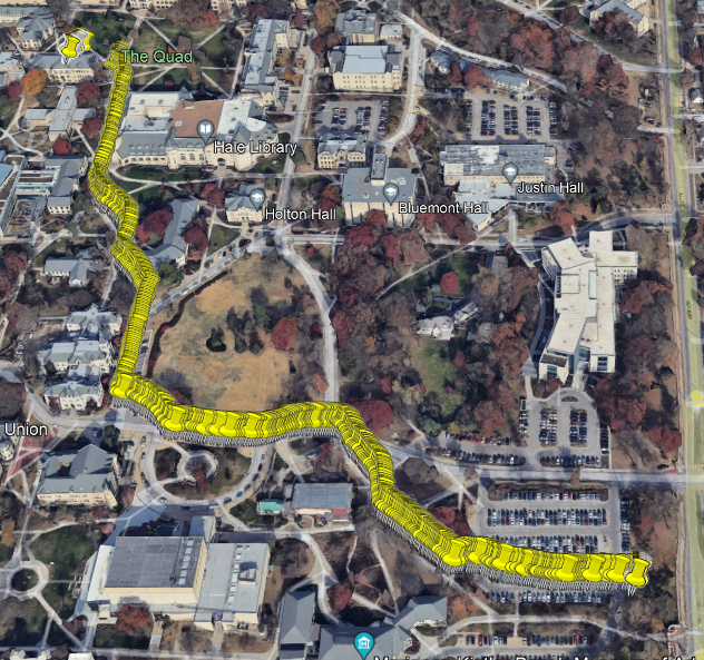
Figure 2.1: Original Route Data
Changing date/time data.
For sf it makes sense to have the data in this class format but I’ve managed to use dplyr in the past to get date/time data to a workable format so long as I didn’t care about GIS work.
Observing the data in it’s current form to make inferences about how to start.
par(mfrow=c(2,1)) puts the two graphs one after the other, it just causes problems if I’m rapid fire pressing ctrl+enter.
# plot time series of spatial locations
par(mfrow=c(2,1))
plot(data.frame(pt.bandlot)[[1]],
     st_coordinates(pt.bandlot)[,1],pch="*",
     xlab="Time",ylab="Longitude")
plot(data.frame(pt.bandlot)[[1]],
     st_coordinates(pt.bandlot)[,2],pch="*",
     xlab="Time",ylab="Lattitude")
# place what we have into a data frame
df.bandlot <- data.frame(time = as.numeric(pt.bandlot$time - pt.bandlot$time[1]),
                         long = st_coordinates(pt.bandlot)[,1],
                         lat = st_coordinates(pt.bandlot)[,2])

head(df.bandlot)
## time long lat
## 1 0 -96.57697 39.18717
## 2 1 -96.57697 39.18718
## 3 2 -96.57697 39.18719
## 4 3 -96.57697 39.18719
## 5 4 -96.57698 39.18719
## 6 5 -96.57699 39.18720Longitude models
The split between longitude and latitude makes sense since all data is being replaced in a prediction frame, separating them into two models and piecing them together in the final product is much more convenient than trying to work with them as a geometric object.
gbm() was the final selection for a model because:
The model needs to handle normally distributed data.
- Long/Lat could be converted to UTM E/N to make them strictly positive.
- Doing that accomplished nothing since Gamma is a bad distribution here.
The model needs to work with my skill level.
- HMM seems like a good option if I understood it better earlier in the course.
- There’s also a package that fits HMM models for animal movement using Gamma and von Mises distributions, but the amount of effort involved in re-configuring the data and building the priors/parameters was outside of my capability.
# maintaining the original lm and gam functions as comparisons
lm1 <- lm(long ~ poly(time,degree=10,raw=TRUE),data=df.bandlot)
gam1 <- gam(long ~ s(time,bs="gp",k=50),data=df.bandlot)
gbm1 <- gbm(long ~ time,data=df.bandlot, distribution="gaussian",n.trees=100, interaction.depth=2, n.minobsinnode=3,shrinkage=.01, bag.fraction=0.1)

summary(lm1)
##
## Call:
## lm(formula = long ~ poly(time, degree = 10, raw = TRUE), data = df.bandlot)
##
## Residuals:
## Min 1Q Median 3Q Max
## -3.262e-04 -1.444e-05 6.400e-07 1.417e-05 2.280e-04
##
## Coefficients:
## Estimate Std. Error t value
## (Intercept) -9.658e+01 1.524e-05 -6.337e+06
## poly(time, degree = 10, raw = TRUE)1 1.424e-05 4.354e-07 3.271e+01
## poly(time, degree = 10, raw = TRUE)2 -1.907e-07 4.064e-09 -4.691e+01
## poly(time, degree = 10, raw = TRUE)3 6.451e-10 1.758e-11 3.670e+01
## poly(time, degree = 10, raw = TRUE)4 -1.182e-12 4.179e-14 -2.829e+01
## poly(time, degree = 10, raw = TRUE)5 1.352e-15 5.961e-17 2.267e+01
## poly(time, degree = 10, raw = TRUE)6 -1.005e-18 5.316e-20 -1.890e+01
## poly(time, degree = 10, raw = TRUE)7 4.848e-22 2.986e-23 1.624e+01
## poly(time, degree = 10, raw = TRUE)8 -1.464e-25 1.026e-26 -1.428e+01
## poly(time, degree = 10, raw = TRUE)9 2.510e-29 1.967e-30 1.276e+01
## poly(time, degree = 10, raw = TRUE)10 -1.865e-33 1.613e-34 -1.156e+01
## Pr(>|t|)
## (Intercept) <2e-16 ***
## poly(time, degree = 10, raw = TRUE)1 <2e-16 ***
## poly(time, degree = 10, raw = TRUE)2 <2e-16 ***
## poly(time, degree = 10, raw = TRUE)3 <2e-16 ***
## poly(time, degree = 10, raw = TRUE)4 <2e-16 ***
## poly(time, degree = 10, raw = TRUE)5 <2e-16 ***
## poly(time, degree = 10, raw = TRUE)6 <2e-16 ***
## poly(time, degree = 10, raw = TRUE)7 <2e-16 ***
## poly(time, degree = 10, raw = TRUE)8 <2e-16 ***
## poly(time, degree = 10, raw = TRUE)9 <2e-16 ***
## poly(time, degree = 10, raw = TRUE)10 <2e-16 ***
## ---
## Signif. codes: 0 '***' 0.001 '**' 0.01 '*' 0.05 '.' 0.1 ' ' 1
##
## Residual standard error: 6.914e-05 on 2405 degrees of freedom
## Multiple R-squared: 0.9976, Adjusted R-squared: 0.9976
## F-statistic: 9.869e+04 on 10 and 2405 DF, p-value: < 2.2e-16##
## Family: gaussian
## Link function: identity
##
## Formula:
## long ~ s(time, bs = "gp", k = 50)
##
## Parametric coefficients:
## Estimate Std. Error t value Pr(>|t|)
## (Intercept) -9.658e+01 1.095e-06 -88240945 <2e-16 ***
## ---
## Signif. codes: 0 '***' 0.001 '**' 0.01 '*' 0.05 '.' 0.1 ' ' 1
##
## Approximate significance of smooth terms:
## edf Ref.df F p-value
## s(time) 20.97 21 77700 <2e-16 ***
## ---
## Signif. codes: 0 '***' 0.001 '**' 0.01 '*' 0.05 '.' 0.1 ' ' 1
##
## Rank: 22/50
## R-sq.(adj) = 0.998 Deviance explained = 99.8%
## GCV = 2.9209e-09 Scale est. = 2.8943e-09 n = 2416Latitude models
# latitude model #

# maintaining the original lm and gam functions as comparisons
lm2 <- lm(lat ~ poly(time,degree=10,raw=TRUE),data=df.bandlot)
gam2 <- gam(lat ~ s(time,bs="gp",k=50),data=df.bandlot)
gbm2 <- gbm(lat ~ time,data=df.bandlot, distribution="gaussian",n.trees=100, interaction.depth=2, n.minobsinnode=3,shrinkage=.01, bag.fraction=0.1)

summary(lm2)
##
## Call:
## lm(formula = lat ~ poly(time, degree = 10, raw = TRUE), data = df.bandlot)
##
## Residuals:
## Min 1Q Median 3Q Max
## -3.623e-04 -3.764e-05 -5.130e-06 2.684e-05 4.234e-04
##
## Coefficients:
## Estimate Std. Error t value
## (Intercept) 3.919e+01 2.481e-05 1.580e+06
## poly(time, degree = 10, raw = TRUE)1 1.149e-05 7.088e-07 1.622e+01
## poly(time, degree = 10, raw = TRUE)2 -1.338e-07 6.616e-09 -2.022e+01
## poly(time, degree = 10, raw = TRUE)3 6.685e-10 2.861e-11 2.336e+01
## poly(time, degree = 10, raw = TRUE)4 -1.487e-12 6.803e-14 -2.185e+01
## poly(time, degree = 10, raw = TRUE)5 1.812e-15 9.703e-17 1.868e+01
## poly(time, degree = 10, raw = TRUE)6 -1.323e-18 8.653e-20 -1.529e+01
## poly(time, degree = 10, raw = TRUE)7 5.933e-22 4.860e-23 1.221e+01
## poly(time, degree = 10, raw = TRUE)8 -1.597e-25 1.669e-26 -9.565e+00
## poly(time, degree = 10, raw = TRUE)9 2.353e-29 3.202e-30 7.349e+00
## poly(time, degree = 10, raw = TRUE)10 -1.446e-33 2.626e-34 -5.508e+00
## Pr(>|t|)
## (Intercept) < 2e-16 ***
## poly(time, degree = 10, raw = TRUE)1 < 2e-16 ***
## poly(time, degree = 10, raw = TRUE)2 < 2e-16 ***
## poly(time, degree = 10, raw = TRUE)3 < 2e-16 ***
## poly(time, degree = 10, raw = TRUE)4 < 2e-16 ***
## poly(time, degree = 10, raw = TRUE)5 < 2e-16 ***
## poly(time, degree = 10, raw = TRUE)6 < 2e-16 ***
## poly(time, degree = 10, raw = TRUE)7 < 2e-16 ***
## poly(time, degree = 10, raw = TRUE)8 < 2e-16 ***
## poly(time, degree = 10, raw = TRUE)9 2.72e-13 ***
## poly(time, degree = 10, raw = TRUE)10 4.03e-08 ***
## ---
## Signif. codes: 0 '***' 0.001 '**' 0.01 '*' 0.05 '.' 0.1 ' ' 1
##
## Residual standard error: 0.0001126 on 2405 degrees of freedom
## Multiple R-squared: 0.994, Adjusted R-squared: 0.994
## F-statistic: 4.018e+04 on 10 and 2405 DF, p-value: < 2.2e-16##
## Family: gaussian
## Link function: identity
##
## Formula:
## lat ~ s(time, bs = "gp", k = 50)
##
## Parametric coefficients:
## Estimate Std. Error t value Pr(>|t|)
## (Intercept) 3.919e+01 9.617e-07 40751591 <2e-16 ***
## ---
## Signif. codes: 0 '***' 0.001 '**' 0.01 '*' 0.05 '.' 0.1 ' ' 1
##
## Approximate significance of smooth terms:
## edf Ref.df F p-value
## s(time) 20.7 21.12 108384 <2e-16 ***
## ---
## Signif. codes: 0 '***' 0.001 '**' 0.01 '*' 0.05 '.' 0.1 ' ' 1
##
## Rank: 24/50
## R-sq.(adj) = 0.999 Deviance explained = 99.9%
## GCV = 2.2547e-09 Scale est. = 2.2345e-09 n = 2416Predictions
The goal is to estimate velocity, although a check for accuracy on location isn’t out of the question.
# lm functions #

# estimate movement trajectory at a very fine temporal scale (every .5s)
df.pred <- data.frame(time = seq(0,2000,by=0.5))
df.pred$long.hat <- predict(lm1,newdata=df.pred)
df.pred$lat.hat <- predict(lm2,newdata=df.pred)

# plot estimated movement trajectory
par(mfrow=c(2,1))
plot(df.bandlot$time,df.bandlot$long,pch="*",xlab="Time",ylab="Longitude")
points(df.pred$time,df.pred$long.hat,typ="l",col="purple",lwd=2)
plot(df.bandlot$time,df.bandlot$lat,pch="*",xlab="Time",ylab="Latitude")
points(df.pred$time,df.pred$lat.hat,typ="l",col="purple",lwd=2)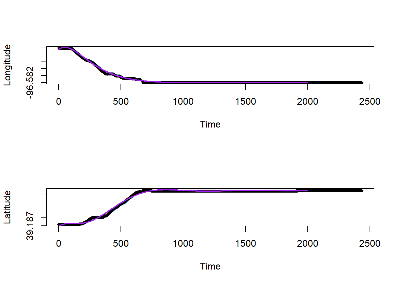
# show time series of estimated speed
pt.bandlot.hat <- st_as_sf(df.pred, coords = c("long.hat", "lat.hat"),
                           crs = st_crs(pt.bandlot))

dist.hat <-
  st_distance(pt.bandlot.hat[1:4000,],pt.bandlot.hat[2:4001,],by_element=TRUE)
(sum(dist.hat)/1000)*0.62
## 0.4976355 [m]# q/a check, estimated trajectory should be in miles at ~0.32
speed.hat <- (dist.hat/0.5)*2.24
# units are in miles/hour
plot(df.pred$time[-1], speed.hat, xlab="Time (seconds)", ylab="Velocity (miles per hour)")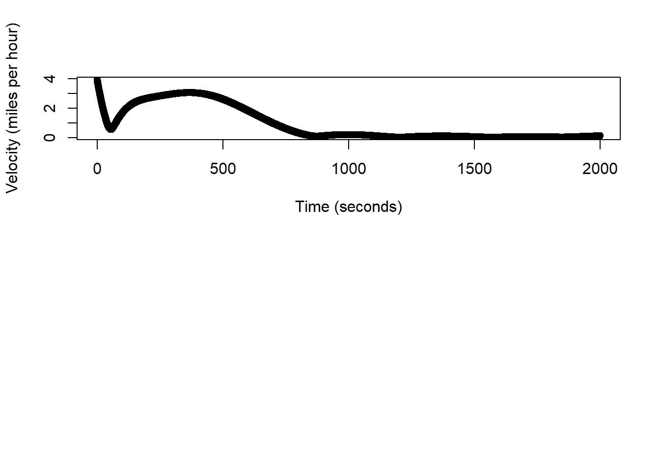
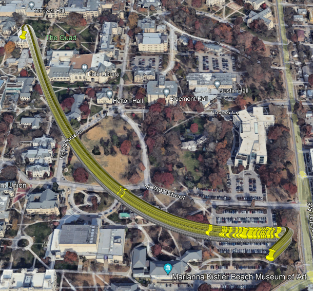
Figure 2.2: Model 1 Predicted Route
# gam functions #

# estimate movement trajectory at a very fine temporal scale (every .5s)
df.pred <- data.frame(time = seq(0,2000,by=0.5))
df.pred$long.hat <- predict(gam1,newdata=df.pred)
df.pred$lat.hat <- predict(gam2,newdata=df.pred)

# plot estimated movement trajectory
par(mfrow=c(2,1))
plot(df.bandlot$time,df.bandlot$long,pch="*",xlab="Time",ylab="Longitude")
points(df.pred$time,df.pred$long.hat,typ="l",col="purple",lwd=2)
plot(df.bandlot$time,df.bandlot$lat,pch="*",xlab="Time",ylab="Latitude")
points(df.pred$time,df.pred$lat.hat,typ="l",col="purple",lwd=2)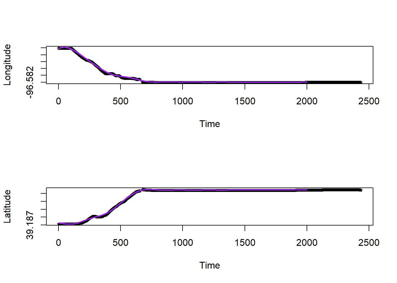
# show time series of estimated speed
pt.bandlot.hat <- st_as_sf(df.pred, coords = c("long.hat", "lat.hat"),
                           crs = st_crs(pt.bandlot))

dist.hat <-
  st_distance(pt.bandlot.hat[1:4000,],pt.bandlot.hat[2:4001,],by_element=TRUE)
(sum(dist.hat)/1000)*0.62
## 0.4847277 [m]# q/a check, estimated trajectory should be in miles at ~0.32
speed.hat <- (dist.hat/0.5)*2.24
# units are in miles/hour
plot(df.pred$time[-1], speed.hat, xlab="Time (seconds)", ylab="Velocity (miles per hour)")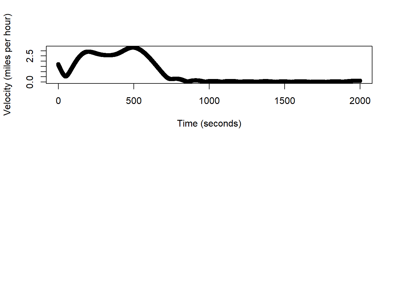
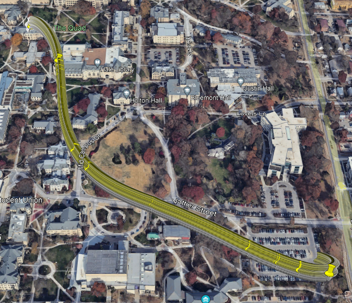
Figure 2.3: Model 2 Predicted Route
# gbm functions #

# estimate movement trajectory at a very fine temporal scale (every .5s)
df.pred <- data.frame(time = seq(0,2000,by=0.5))
df.pred$long.hat <- predict(gbm1,newdata=df.pred)
## Using 100 trees...## Using 100 trees...# plot estimated movement trajectory
par(mfrow=c(2,1))
plot(df.bandlot$time,df.bandlot$long,pch="*",xlab="Time",ylab="Longitude")
points(df.pred$time,df.pred$long.hat,typ="l",col="purple",lwd=2)
plot(df.bandlot$time,df.bandlot$lat,pch="*",xlab="Time",ylab="Latitude")
points(df.pred$time,df.pred$lat.hat,typ="l",col="purple",lwd=2)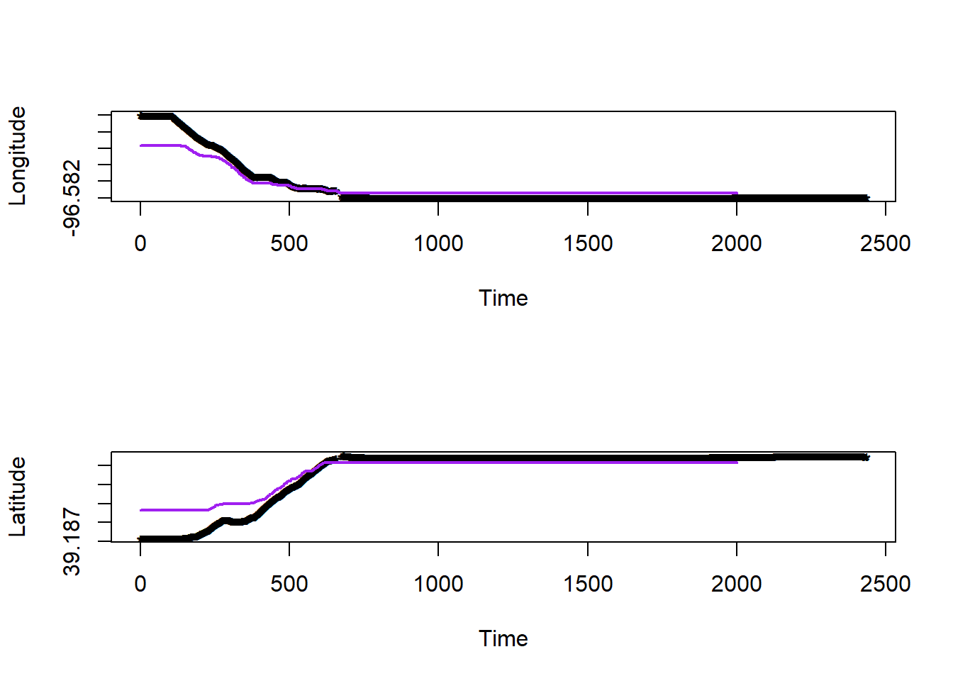
# show time series of estimated speed
pt.bandlot.hat <- st_as_sf(df.pred, coords = c("long.hat", "lat.hat"),
                           crs = st_crs(pt.bandlot))

dist.hat <-
  st_distance(pt.bandlot.hat[1:4000,],pt.bandlot.hat[2:4001,],by_element=TRUE)
(sum(dist.hat)/1000)*0.62
## 0.3213426 [m]# q/a check, estimated trajectory should be in miles at ~0.32
speed.hat <- (dist.hat/0.5)*2.24
# units are in miles/hour
plot(df.pred$time[-1], speed.hat, xlab="Time (seconds)", ylab="Velocity (miles per hour)")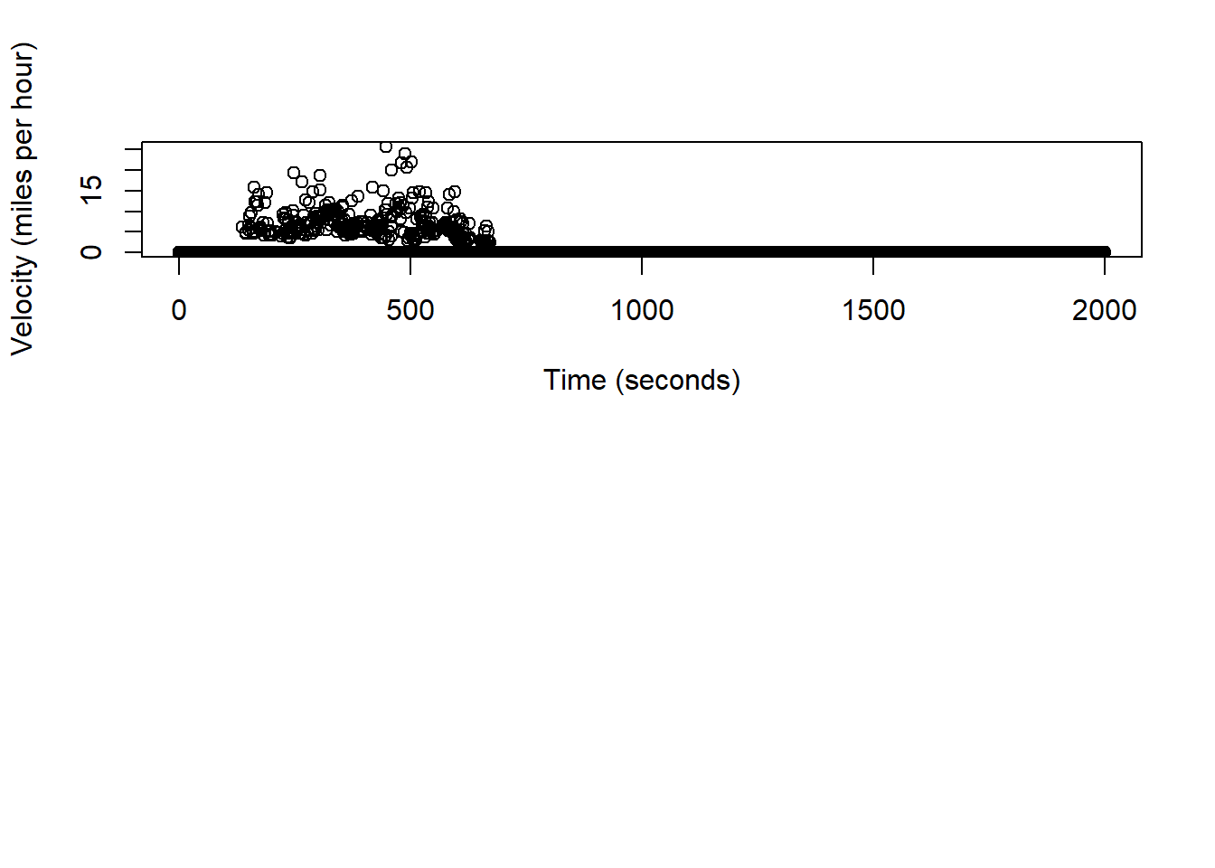
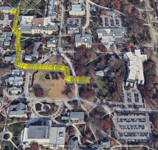
Figure 2.4: Model 3 Predicted Route
For the purpose of getting the bookdown to work, the code creating the .kml file had to be left out of the functional code blocks. I’ve left it below for reference that everything was visualized: