Chapter 3 Assignment 2
Data Prep
Package Explanations:
sf: GIS work in R
sp: additional spatial stats features
raster: allows working with raster files in R (more GIS software)
fields: even more spatial tools
dplyr: data prep/cleaning
stringr: final data presentation, helps with making tables
rsample: for re-sampling data later on
gbm: contains the
gbm()function (gradient boosted regression ML)rpart: contains the
rpart()function (recursive partinition ML)
The raw data from Strava of my walk across the field in front of Anderson hall (I definitely looked insane), and the standard Kansas shapefile.
# dropbox of spatial data
url <-
  "https://www.dropbox.com/scl/fi/0jv0p7advzw2b4nl7j8zc/Spatial_data_of_Anderson_green.gpx?rlkey=xp28o3cbbq5jljo29vkxcwc9w&dl=1"

# read the file
pt.and <- st_read(dsn=url,layer="track_points")
## Reading layer `track_points' from data source
## `https://www.dropbox.com/scl/fi/0jv0p7advzw2b4nl7j8zc/Spatial_data_of_Anderson_green.gpx?rlkey=xp28o3cbbq5jljo29vkxcwc9w&dl=1'
## using driver `GPX'
## Simple feature collection with 1661 features and 26 fields
## Geometry type: POINT
## Dimension: XY
## Bounding box: xmin: -96.58064 ymin: 39.18812 xmax: -96.57917 ymax: 39.18956
## Geodetic CRS: WGS 84# keep only spatial data
pt.and <- pt.and[,4]
# load shapefile of Kansas from census.gov
sf.us <- st_read("cb_2015_us_state_20m.shp")## Reading layer `cb_2015_us_state_20m' from data source
## `C:\Users\rmsho\Documents\ST764-Portfolio\Portfolio-Sholl\cb_2015_us_state_20m.shp'
## using driver `ESRI Shapefile'
## Simple feature collection with 52 features and 9 fields
## Geometry type: MULTIPOLYGON
## Dimension: XY
## Bounding box: xmin: -179.1743 ymin: 17.91377 xmax: 179.7739 ymax: 71.35256
## Geodetic CRS: NAD83sf.kansas <- sf.us[48,6]
sf.kansas <- as(sf.kansas, 'Spatial')
# Plot to confirm the correct file has been pulled
plot(sf.kansas,main="",col="white")
Shapefile of Anderson field for a boundary of the map.
I actually didn’t record a separate walk around the perimeter and eliciting the perimeter from my initial data sounded painful, fortunately Yoshi was already working on the same area for his project so I “borrowed” his file. Industry gold-standard behavior.
# Make shapefile of study area around Anderson green
## (credits: Yoshimitsu Nagaoka)
url <-
  "https://www.dropbox.com/scl/fi/rjsmyq7tfmabin0fkh8q4/Boundary-3-1.gpx?rlkey=87difl7j4nonaewlde4ngzd0q&dl=1"
pt.study.area <- st_read(dsn=url,layer="track_points")
## Reading layer `track_points' from data source
## `https://www.dropbox.com/scl/fi/rjsmyq7tfmabin0fkh8q4/Boundary-3-1.gpx?rlkey=87difl7j4nonaewlde4ngzd0q&dl=1'
## using driver `GPX'
## Simple feature collection with 443 features and 26 fields
## Geometry type: POINT
## Dimension: XY
## Bounding box: xmin: -96.5807 ymin: 39.18817 xmax: -96.57913 ymax: 39.18952
## Geodetic CRS: WGS 84sf.study.area <- st_polygon(list(rbind(st_coordinates(pt.study.area),st_coordinates(pt.study.area)[1,])))
sf.study.area <- st_buffer(sf.study.area, .00006)
sf.study.area <- st_sf(st_sfc(sf.study.area),crs = crs(sf.kansas))
plot(sf.study.area)
plot(pt.and,add=TRUE)
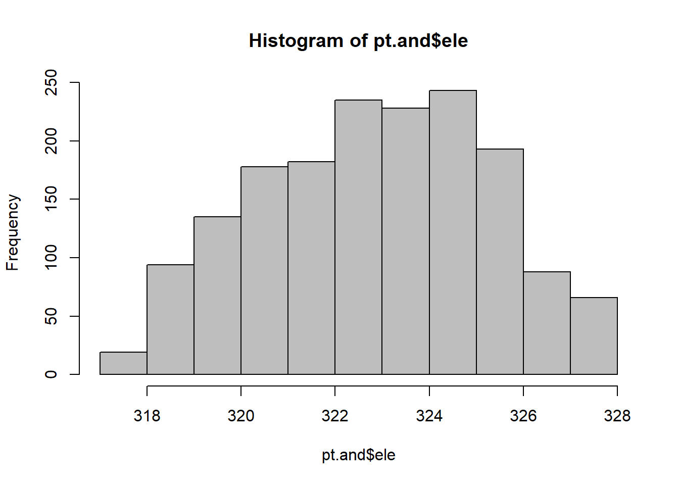
##    Min. 1st Qu.  Median    Mean 3rd Qu.    Max.
##   317.6   321.0   323.0   322.9   324.7   327.5
# Transform pointfiles and shapefiles to utm zone to a planar coordinate reference system
pt.and.utm <- st_transform(pt.and,CRS("+proj=utm +zone=14 +datum=WGS84 +units=m"))
sf.study.area.utm <- st_transform(sf.study.area,CRS("+proj=utm +zone=14 +datum=WGS84 +units=m"))Final step of the process was producing a data frame of the points and doing a split of the data. I attempted to split the data for the models and work with it exclusively split, which has worked in the past but didn’t work here. So the split is for a model check at the end.
# build data frame out of pointfiles
df.and <- data.frame (elev = pt.and$ele,
                          long = st_coordinates(pt.and)[,1],
                          lat = st_coordinates(pt.and)[,2],
                          s1 = st_coordinates(pt.and.utm)[,1],
                          s2 = st_coordinates(pt.and.utm)[,2])


# preparing split for interpolation

df.split <- df.and %>% mutate_if(is.ordered, factor,ordered = FALSE)

# seed for reproducibility

set.seed(73)

and_split <- initial_split(df.split, prop = .7, strata = "elev")
and_train <- training(and_split)
and_test  <- testing(and_split)
Models
Goals:
Produce an accurate prediction of elevation at every point within my data
Compare the accuracy gain from using a generalized linear model versus applying a machine learning algorithm to the exact same model.
The major intent is to uncover the realistic use case of using machine learning. In my experience machine learning is a commonality to allow automation of processes that would otherwise demand multiple hours of an employee’s week. With statistics it seems their major usage is finding higher accuracy predictions by training a model.
So far with machine learning I’ve encountered the major issue of it being difficult to check the model efficacy outside of very basic methods like graphical diagnostics and within-sample validation. Other methods of obtaining predictions can quantify uncertainty much more reliably.
All three of our functions are the same generalize model:
\[
y_i = \beta_0 + \beta_{s1} + \beta_{s2} + \epsilon_i
\]
Our gradient boosted tree uses a semi-complex algorithm to minimize meean squared error across \(m\) iterations (displayed as n.trees in the actual gbm() function syntax).
Space is continuous for the purpose of this project, and recursive partitioning has a problem with over fitting continuous data. That said, we’ll be using it as a comparison tool.
Recursive partitioning is less about minimizing mean squared error specifically, and instead focuses on running all possible decision trees until they have reached a certain failure condition. A proper decision path is created out of these failure iterations until a rapid and accurate end product is produced. This is why over fitting of continuous data is a problem with the model, since it will generate decision trees for all the continuous points and end up generating a very accurate result with no forecasting capabilities.
GLM
set.seed(73)

m1 <- glm(elev ~ s1 + s2,family = "gaussian",data = df.and)

# make raster of study area to be able to map predictions from models
rl.andp.a <- raster(,nrow=100,ncols=100,ext=extent(sf.study.area.utm),crs=crs(sf.study.area.utm))


# make data frame to be able to make predictions at each pixel (cell of raster)
df.pred <- data.frame(elev = NA,
                      s1 = xyFromCell(rl.andp.a,cell=1:length(rl.andp.a[]))[,1],
                      s2 = xyFromCell(rl.andp.a,cell=1:length(rl.andp.a[]))[,2])

# make spatial predictions at each pixel
df.pred$elev <- predict(m1,newdata=df.pred)

# view first 6 rows of predictions
head(df.pred)
## elev s1 s2
## 1 329.5910 708942.4 4340604
## 2 329.4962 708943.8 4340604
## 3 329.4013 708945.3 4340604
## 4 329.3065 708946.8 4340604
## 5 329.2117 708948.2 4340604
## 6 329.1169 708949.7 4340604# fill raster file with predictions
rl.andp.a[] <- df.pred$elev
rl.andp.a <- mask(rl.andp.a,sf.study.area.utm)
# plot map of predictions
plot(rl.andp.a)
plot(sf.study.area.utm,add=TRUE)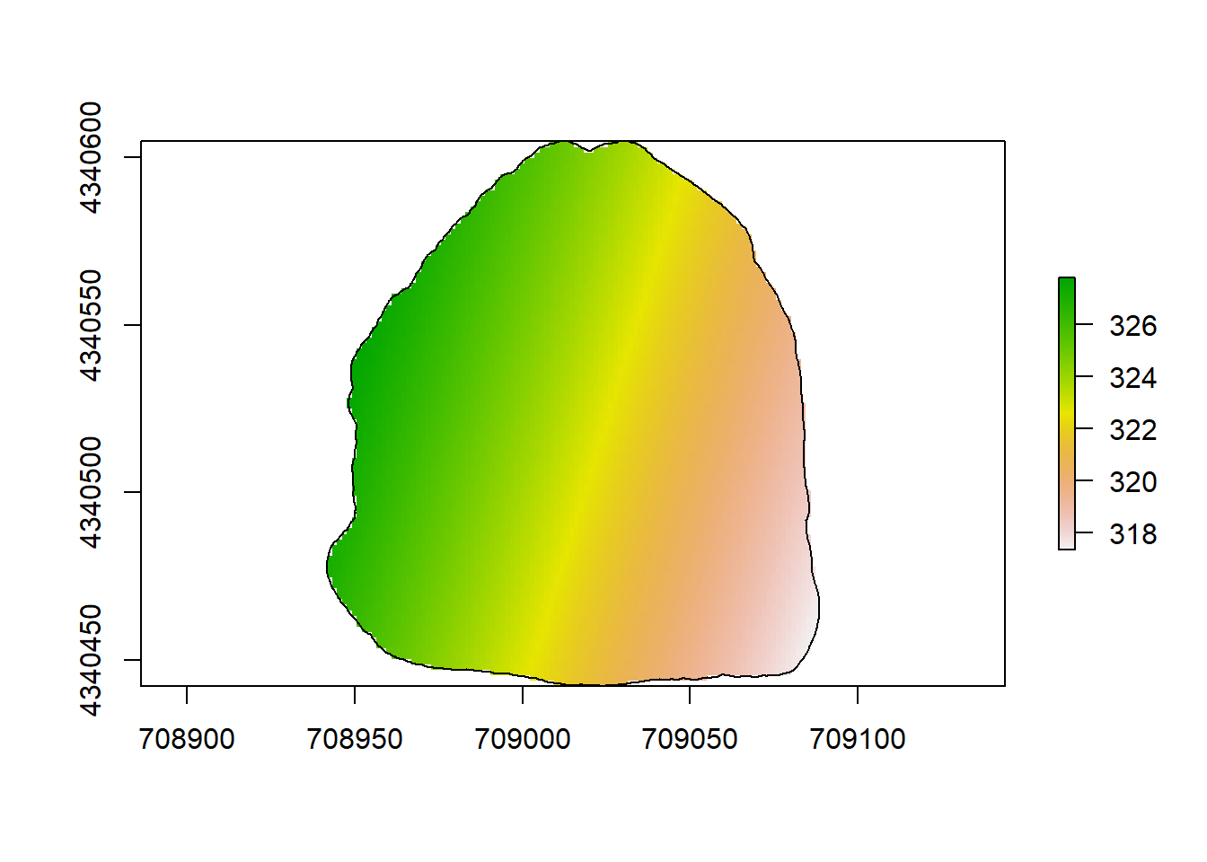
GBM
set.seed(73)

m2 <- gbm(elev ~ s1 + s2, data = df.and, n.trees=1000, interaction.depth=2, n.minobsinnode=3, shrinkage=.01, bag.fraction=0.1)
## Distribution not specified, assuming gaussian ...# make raster of study area to be able to map predictions from models
rl.andp.b <- raster(,nrow=100,ncols=100,ext=extent(sf.study.area.utm),crs=crs(sf.study.area.utm))
# make data frame to be able to make predictions at each pixel (cell of raster)
df.pred2 <- data.frame(elev = NA,
s1 = xyFromCell(rl.andp.b,cell=1:length(rl.andp.b[]))[,1],
s2 = xyFromCell(rl.andp.b,cell=1:length(rl.andp.b[]))[,2])
# make spatial predictions at each pixel
df.pred2$elev <- predict(m2,newdata=df.pred2) ## Using 1000 trees...## elev s1 s2
## 1 328.6809 708942.4 4340604
## 2 328.6809 708943.8 4340604
## 3 328.6809 708945.3 4340604
## 4 328.6809 708946.8 4340604
## 5 328.6809 708948.2 4340604
## 6 328.6809 708949.7 4340604# fill raster file with predictions
rl.andp.b[] <- df.pred2$elev
rl.andp.b <- mask(rl.andp.b,sf.study.area.utm)
# plot map of predictions
plot(rl.andp.b)
plot(sf.study.area.utm,add=TRUE)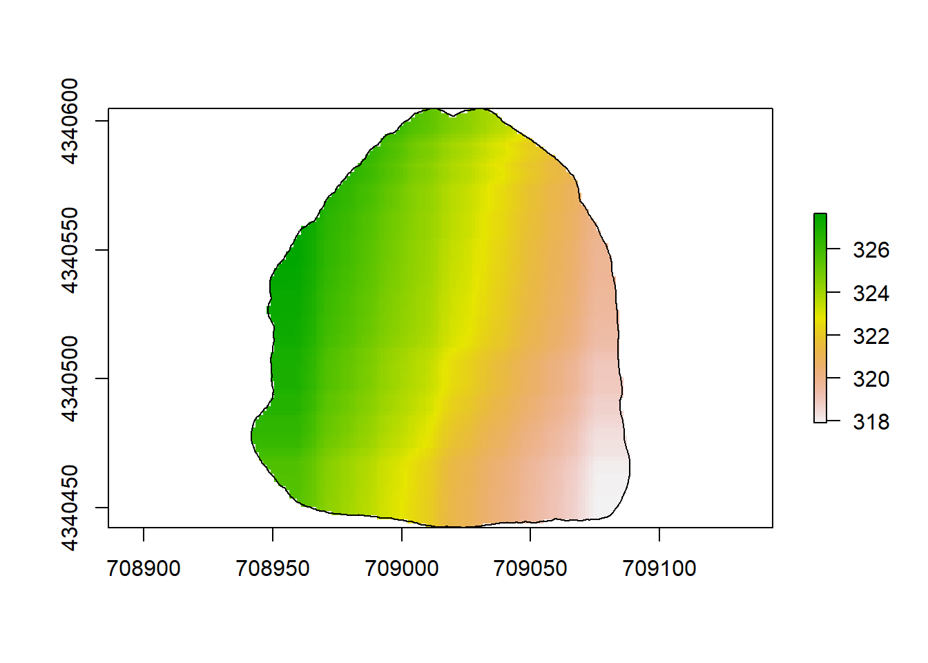
RPART
set.seed(73)

m3 <- rpart(elev ~ s1 + s2, data = df.and , control = rpart.control(cp = 0.0001))

# make raster of study area to be able to map predictions from models
rl.andp.c <- raster(,nrow=100,ncols=100,ext=extent(sf.study.area.utm),crs=crs(sf.study.area.utm))


# make data frame to be able to make predictions at each pixel (cell of raster)
df.pred3 <- data.frame(elev = NA,
                      s1 = xyFromCell(rl.andp.c,cell=1:length(rl.andp.c[]))[,1],
                      s2 = xyFromCell(rl.andp.c,cell=1:length(rl.andp.c[]))[,2])

# make spatial predictions at each pixel
df.pred3$elev <- predict(m3,newdata=df.pred3)

# view first 6 rows of predictions
head(df.pred3)
## elev s1 s2
## 1 327.3596 708942.4 4340604
## 2 327.3596 708943.8 4340604
## 3 327.3596 708945.3 4340604
## 4 327.3596 708946.8 4340604
## 5 327.3596 708948.2 4340604
## 6 327.3596 708949.7 4340604# fill raster file with predictions
rl.andp.c[] <- df.pred3$elev
rl.andp.c <- mask(rl.andp.c,sf.study.area.utm)
# plot map of predictions
plot(rl.andp.c)
plot(sf.study.area.utm,add=TRUE)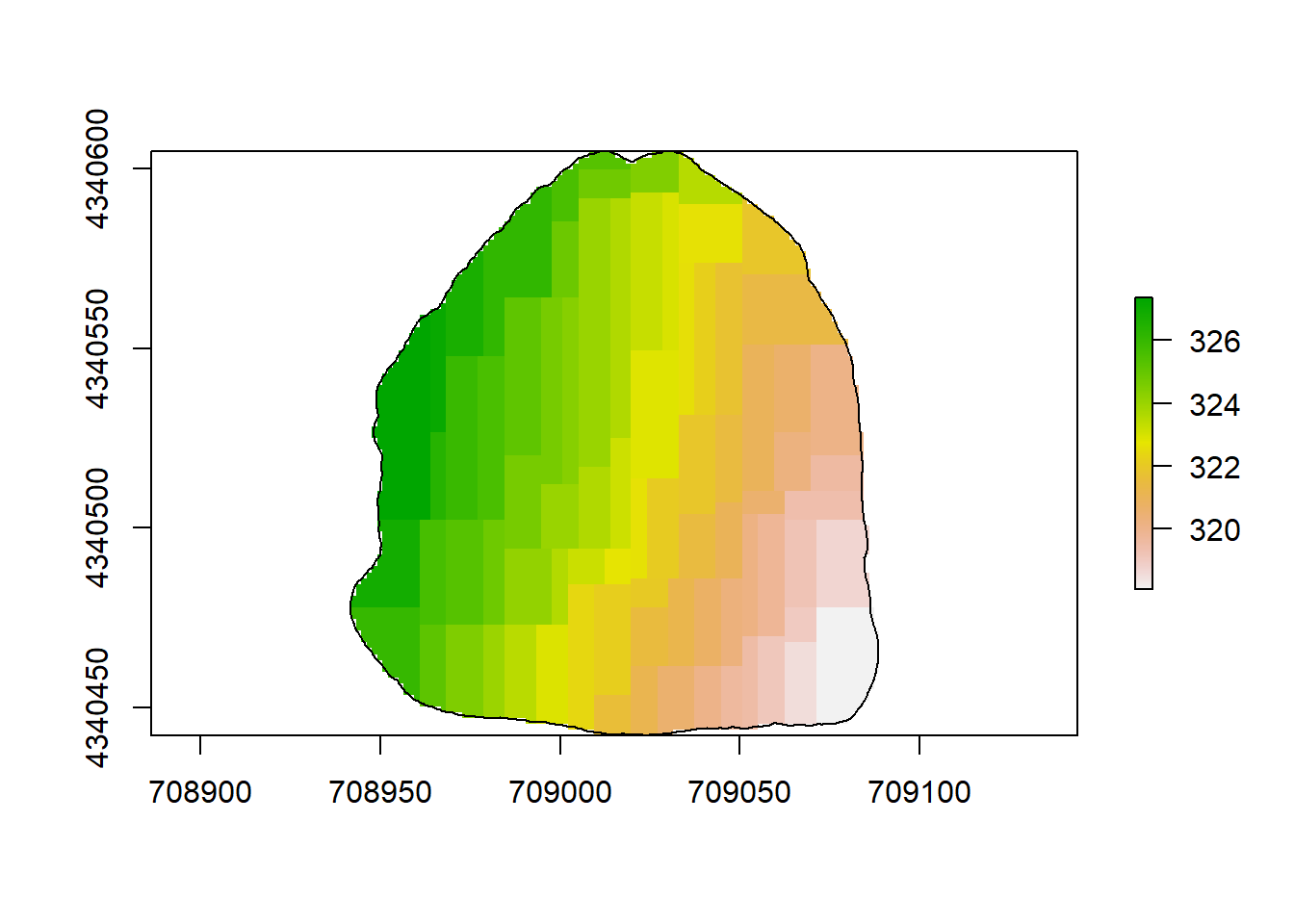
Model Checks
Originally, how I did this portion was not very elegant. I’ve since gone back and made use of the method of performing within-sample validation that I learned for the final project.
set.seed(73)

m1.int <- glm(elev ~ s1 + s2,family = "gaussian",data = and_train)

int_pred.m1 <- predict(m1, newdata = and_test, type = "response")
mspe.m1.int <- sum((int_pred.m1 - and_test$elev)^2)

m2.int <- gbm(elev ~ s1 + s2, data = and_train)
## Distribution not specified, assuming gaussian ...## Using 1000 trees...mspe.m2.int <- sum((int_pred.m2 - and_test$elev)^2)
m3.int <- rpart(elev ~ s1 + s2, data = and_train, control = rpart.control(cp = 0.0001))
int_pred.m3 <- predict(m3, newdata = and_test, type = "vector")
mspe.m3.int <- sum((int_pred.m3 - and_test$elev)^2)With the last step finalized, I can make inferences about quality for each model.


n.models <- c("GLM","GBM","RPART")
models <- str_wrap(n.models, width = 15)
MSPE <- c(mspe.m1.int,mspe.m2.int,mspe.m3.int)
Table_MSPE <- data.frame(models, MSPE)
print(Table_MSPE)
## models MSPE
## 1 GLM 33.74986
## 2 GBM 18.70639
## 3 RPART 22.77651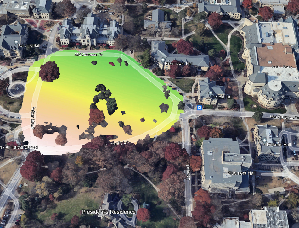
(#fig:a2.image1)GLM Map
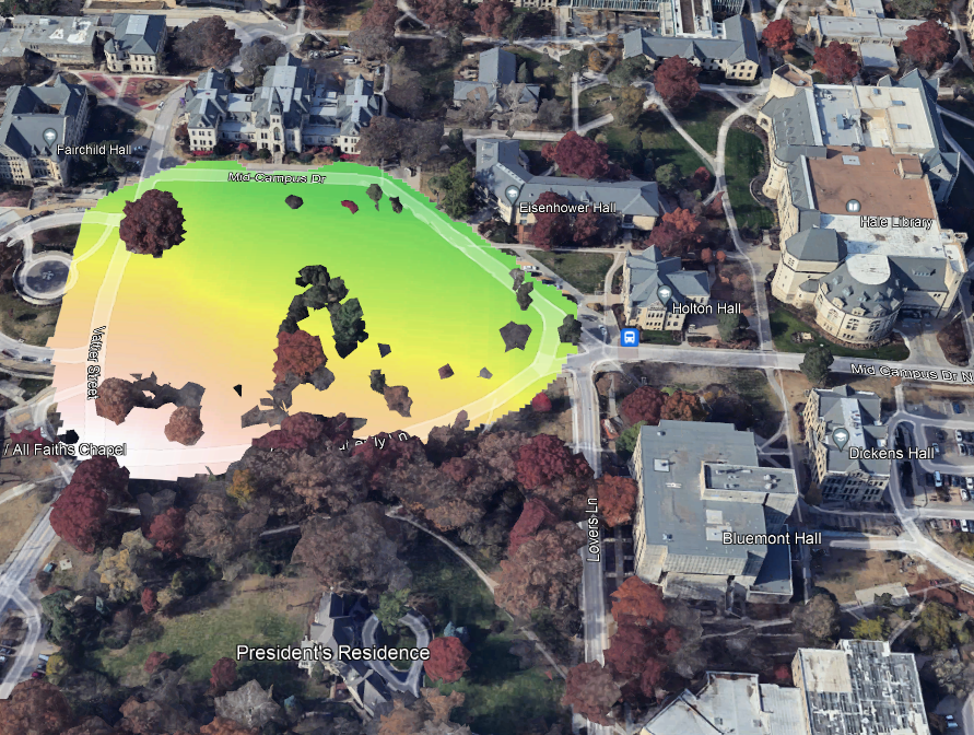
(#fig:a2.image2)GBM Map
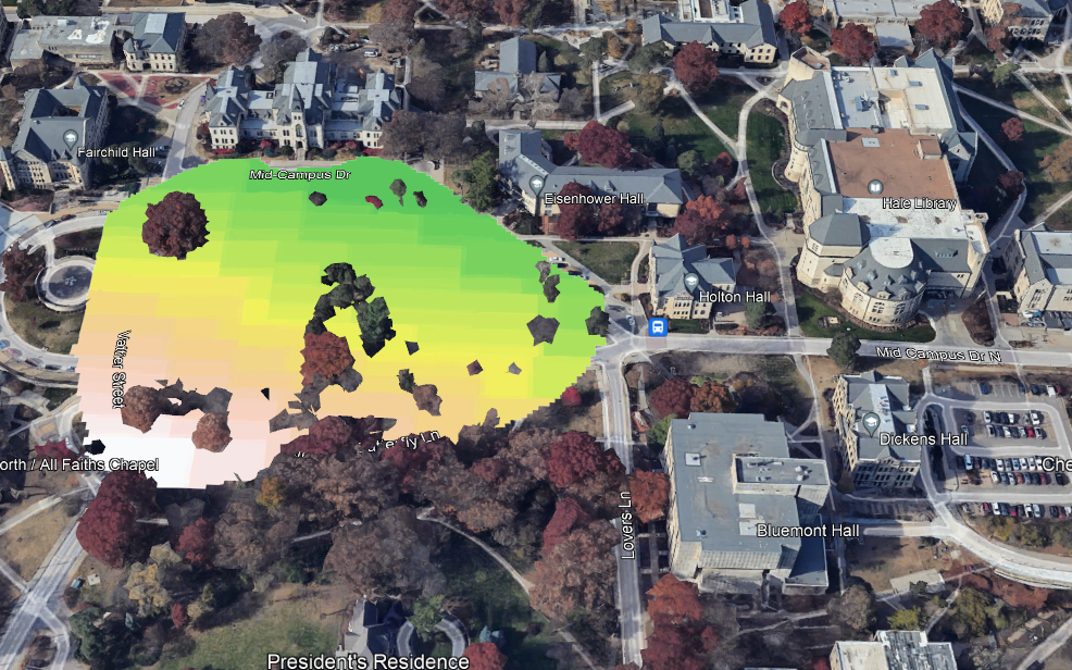
(#fig:a2.image3)RPART Map