22 Parallel Computation
Many computations in R can be made faster by the use of parallel computation. Generally, parallel computation is the simultaneous execution of different pieces of a larger computation across multiple computing processors or cores. The basic idea is that if you can execute a computation in \(X\) seconds on a single processor, then you should be able to execute it in \(X/n\) seconds on \(n\) processors. Such a speed-up is generally not possible because of overhead and various barriers to splitting up a problem into \(n\) pieces, but it is often possible to come close in simple problems.
It used to be that parallel computation was squarely in the domain of “high-performance computing”, where expensive machines were linked together via high-speed networking to create large clusters of computers. In those kinds of settings, it was important to have sophisticated software to manage the communication of data between different computers in the cluster. Parallel computing in that setting was a highly tuned, and carefully customized operation and not something you could just saunter into.
These days though, almost all computers contain multiple processors or cores on them. Even Apple’s iPhone 6S comes with a dual-core CPU as part of its A9 system-on-a-chip. Getting access to a “cluster” of CPUs, in this case all built into the same computer, is much easier than it used to be and this has opened the door to parallel computing for a wide range of people.
In this chapter, we will discuss some of the basic funtionality in R for executing parallel computations. In particular, we will focus on functions that can be used on multi-core computers, which these days is almost all computers. It is possible to do more traditional parallel computing via the network-of-workstations style of computing, but we will not discuss that here.
22.2 Embarrassing Parallelism
Many problems in statistics and data science can be executed in an “embarrassingly parallel” way, whereby multiple independent pieces of a problem are executed simultaneously because the different pieces of the problem never really have to communicate with each other (except perhaps at the end when all the results are assembled). Despite the name, there’s nothing really “embarrassing” about taking advantage of the structure of the problem and using it speed up your computation. In fact, embarrassingly parallel computation is a common paradigm in statistics and data science.
In general, it is NOT a good idea to use the functions described in
this chapter with graphical user interfaces (GUIs) because, to summarize
the help page for mclapply(), bad things can happen. That
said, the functions in the parallel package seem two work
okay in RStudio.
The basic mode of an embarrassingly parallel operation can be seen with the lapply() function, which we have reviewed in a previous chapter. Recall that the lapply() function has two arguments:
A list, or an object that can be coerced to a list.
A function to be applied to each element of the list
Finally, recall that lapply() always returns a list whose length is equal to the length of the input list.
The lapply() function works much like a loop–it cycles through each element of the list and applies the supplied function to that element. While lapply() is applying your function to a list element, the other elements of the list are just…sitting around in memory. Note that in the description of lapply() above, there’s no mention of the different elements of the list communicating with each other, and the function being applied to a given list element does not need to know about other list elements.
Just about any operation that is handled by the lapply() function can be parallelized. This approach is analogous to the “map-reduce” approach in large-scale cluster systems. The idea is that a list object can be split across multiple cores of a processor and then the function can be applied to each subset of the list object on each of the cores. Conceptually, the steps in the parallel procedure are
Split list
Xacross multiple coresCopy the supplied function (and associated environment) to each of the cores
Apply the supplied function to each subset of the list
Xon each of the cores in parallelAssemble the results of all the function evaluations into a single list and return
The differences between the many packages/functions in R essentially come down to how each of these steps are implemented. In this chapter we will cover the parallel package, which has a few implementations of this paradigm. The goal of the functions in this package (and in other related packages) is to abstract the complexities of the implemetation so that the R user is presented a relatively clean interface for doing computations.
22.3 The Parallel Package
The parallel package which comes with your R installation. It represents a combining of two historical packages–the multicore and snow packages, and the functions in parallel have overlapping names with those older packages. For our purposes, it’s not necessary to know anything about the multicore or snow packages, but long-time users of R may remember them from back in the day.
The mclapply() function essentially parallelizes calls to lapply(). The first two arguments to mclapply() are exactly the same as they are for lapply(). However, mclapply() has further arguments (that must be named), the most important of which is the mc.cores argument which you can use to specify the number of processors/cores you want to split the computation across. For example, if your machine has 4 cores on it, you might specify mc.cores = 4 to break your parallelize your operation across 4 cores (although this may not be the best idea if you are running other operations in the background besides R).
The mclapply() function (and related mc* functions) works via the fork mechanism on Unix-style operating systems. Briefly, your R session is the main process and when you call a function like mclapply(), you fork a series of sub-processes that operate independently from the main process (although they share a few low-level features). These sub-processes then execute your function on their subsets of the data, presumably on separate cores of your CPU. Once the computation is complete, each sub-process returns its results and then the sub-process is killed. The parallel package manages the logistics of forking the sub-processes and handling them once they’ve finished.
Because of the use of the fork mechanism, the mc*
functions are generally not available to users of the Windows operating
system.
The first thing you might want to check with the parallel package is if your computer in fact has multiple cores that you can take advantage of.
> library(parallel)
> detectCores()
[1] 16
The computer on which this is being written is a circa 2016 MacBook Pro (with Touch Bar) with 2 physical CPUs. However, because each core allows for hyperthreading, each core is presented as 2 separate cores, allowing for 4 “logical” cores. This is what detectCores() returns. On some systems you can call detectCores(logical = FALSE) to return the number of physical cores.
> detectCores(logical = FALSE)  ## Same answer as before on some systems?
[1] 8
In general, the information from detectCores() should be used cautiously as obtaining this kind of information from Unix-like operating systems is not always reliable. If you are going down this road, it’s best if you get to know your hardware better in order to have an understanding of how many CPUs/cores are available to you.
22.3.1 mclapply()
The simplest application of the parallel package is via the mclapply() function, which conceptually splits what might be a call to lapply() across multiple cores. Just to show how the function works, I’ll run some code that splits a job across 10 cores and then just sleeps for 10 seconds.
> r <- mclapply(1:10, function(i) {
+         Sys.sleep(10)  ## Do nothing for 10 seconds
+ }, mc.cores = 10)      ## Split this job across 10 cores
While this “job” was running, I took a screen shot of the system activity monitor (“top”). Here’s what it looks like on Mac OS X.

Multiple sub-processes spawned by mclapply()
In case you are not used to viewing this output, each row of the table is an application or process running on your computer. You can see that there are 11 rows where the COMMAND is labelled rsession. One of these is my primary R session (being run through RStudio), and the other 10 are the sub-processes spawned by the mclapply() function.
We will use as a second (slightly more realistic) example processing data from multiple files. Often this is something that can be easily parallelized.
Here we have data on ambient concentrations of sulfate particulate matter (PM) and nitrate PM from 332 monitors around the United States. First, we can read in the data via a simple call to lapply().
> infiles <- dir("specdata", full.names = TRUE)
> specdata <- lapply(infiles, read.csv)
Now, specdata is a list of data frames, with each data frame corresponding to each of the 332 monitors in the dataset.
One thing we might want to do is compute a summary statistic across each of the monitors. For example, we might want to compute the 90th percentile of sulfate for each of the monitors. This can easily be implemented as a serial call to lapply().
> s <- system.time({
+         mn <- lapply(specdata, function(df) {
+                 quantile(df$sulfate, 0.9, na.rm = TRUE)
+         })
+ })
> s
   user  system elapsed
  0.034   0.000   0.034
Note that in the system.time() output, the user time (0.034 seconds) and the elapsed time (0.034 seconds) are roughly the same, which is what we would expect because there was no parallelization.
The equivalent call using mclapply() would be
> s <- system.time({
+         mn <- mclapply(specdata, function(df) {
+                 quantile(df$sulfate, 0.9, na.rm = TRUE)
+         }, mc.cores = 4)
+ })
> s
   user  system elapsed
  0.002   0.004   0.027
You’ll notice that the the elapsed time is now less than the user time. However, in general, the elapsed time will not be 1/4th of the user time, which is what we might expect with 4 cores if there were a perfect performance gain from parallelization.
R keeps track of how much time is spent in the main process and how much is spent in any child processes.
> s["user.self"]  ## Main process
user.self
    0.002
> s["user.child"] ## Child processes
user.child
         0
In the call to mclapply() you can see that virtually all of the user time is spent in the child processes. The total user time is the sum of the self and child times.
In some cases it is possible for the parallelized version of an R expression to actually be slower than the serial version. This can occur if there is substantial overhead in creating the child processes. For example, time must be spent copying information over to the child processes and communicating the results back to the parent process. However, for most substantial computations, there will be some benefit in parallelization.
One advantage of serial computations is that it allows you to better
keep a handle on how much memory your R job is using.
When executing parallel jobs via mclapply() it’s important
to pre-calculate how much memory all of the processes will
require and make sure this is less than the total amount of memory on
your computer.
The mclapply() function is useful for iterating over a single list or list-like object. If you have to iterate over multiple objects together, you can use mcmapply(), which is the the multi-core equivalent of the mapply() function.
22.3.2 Error Handling
When either mclapply() or mcmapply() are called, the functions supplied will be run in the sub-process while effectively being wrapped in a call to try(). This allows for one of the sub-processes to fail without disrupting the entire call to mclapply(), possibly causing you to lose much of your work. If one sub-process fails, it may be that all of the others work just fine and produce good results.
This error handling behavior is a significant difference from the usual call to lapply(). With lapply(), if the supplied function fails on one component of the list, the entire function call to lapply() fails and you only get an error as a result.
With mclapply(), when a sub-process fails, the return value for that sub-process will be an R object that inherits from the class "try-error", which is something you can test with the inherits() function. Conceptually, each child process is executed with the try() function wrapped around it. The code below deliberately causes an error in the 3 element of the list.
> r <- mclapply(1:5, function(i) {
+         if(i == 3L)
+                 stop("error in this process!")
+         else
+                 return("success!")
+ }, mc.cores = 5)
Warning in mclapply(1:5, function(i) {: scheduled core 3 encountered error in
user code, all values of the job will be affected
Here we see there was a warning but no error in the running of the above code. We can check the return value.
> str(r)
List of 5
 $ : chr "success!"
 $ : chr "success!"
 $ : 'try-error' chr "Error in FUN(X[[i]], ...) : error in this process!\n"
  ..- attr(*, "condition")=List of 2
  .. ..$ message: chr "error in this process!"
  .. ..$ call   : language FUN(X[[i]], ...)
  .. ..- attr(*, "class")= chr [1:3] "simpleError" "error" "condition"
 $ : chr "success!"
 $ : chr "success!"
Note that the 3rd list element in r is different.
> class(r[[3]])
[1] "try-error"
> inherits(r[[3]], "try-error")
[1] TRUE
When running code where there may be errors in some of the sub-processes, it’s useful to check afterwards to see if there are any errors in the output received.
> bad <- sapply(r, inherits, what = "try-error")
> bad
[1] FALSE FALSE  TRUE FALSE FALSE
You can subsequently subset your return object to only keep the “good” elements.
> r.good <- r[!bad]
> str(r.good)
List of 4
 $ : chr "success!"
 $ : chr "success!"
 $ : chr "success!"
 $ : chr "success!"
22.4 Example: Bootstrapping a Statistic
One technique that is commonly used to assess the variability of a statistic is the bootstrap. Briefly, the bootstrap technique resamples the original dataset with replacement to create pseudo-datasets that are similar to, but slightly perturbed from, the original dataset. This technique is particularly useful when the statistic in question does not have a readily accessible formula for its standard error.
One example of a statistic for which the bootstrap is useful is the median. Here, we plot the histogram of some of the sulfate particulate matter data from the previous example.
> dat <- read.csv("specdata/001.csv")
> sulf <- dat$sulfate
> sulf <- sulf[!is.na(sulf)]     ## Remove missing values
> hist(sulf, xlab = expression("Sulfate PM (" * mu * g/m^3 * ")"))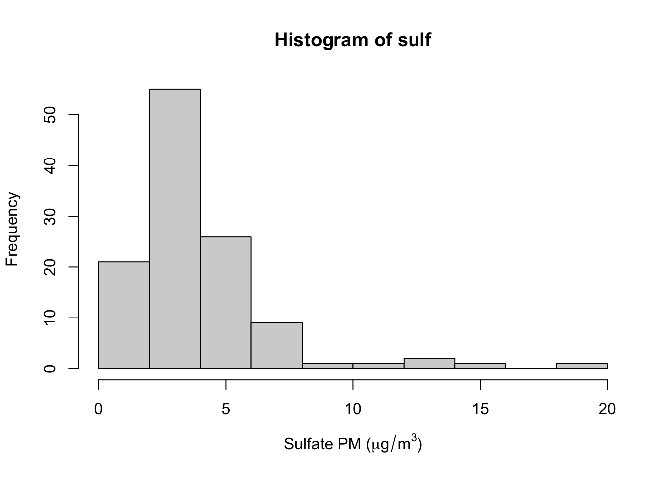
We can see from the histogram that the distribution of sulfate is skewed to the right. Therefore, it would seem that the median might be a better summary of the distribution than the mean.
> summary(sulf)
   Min. 1st Qu.  Median    Mean 3rd Qu.    Max.
  0.613   2.210   2.870   3.881   4.730  19.100
How can we construct confidence interval for the median of sulfate for this monitor? The bootstrap is simple procedure that can work well. Here’s how we might do it in the usual (non-parallel) way.
> set.seed(1)
> med.boot <- replicate(5000, {
+         xnew <- sample(sulf, replace = TRUE)
+         median(xnew)
+ })
A 95% confidence interval would then take the 2.5th and 97.5th percentiles of this distribution (this is known as the percentile method).
> quantile(med.boot, c(0.025, 0.975))
 2.5% 97.5%
 2.70  3.47
How could be done in parallel? We could simply wrap the expression passed to replicate() in a function and pass it to mclapply(). However, one thing we need to be careful of is generating random numbers.
22.4.1 Generating Random Numbers
Generating random numbers in a parallel environment warrants caution because it’s possible to create a situation where each of the sub-processes are all generating the exact same random numbers. For the most part, the mc* functions do their best to avoid this.
> r <- mclapply(1:5, function(i) {
+         rnorm(3)
+ }, mc.cores = 5)
> str(r)
List of 5
 $ : num [1:3] -0.7308 -0.5486 0.0307
 $ : num [1:3] 0.258 -1.028 0.81
 $ : num [1:3] -0.526 -0.477 -0.671
 $ : num [1:3] 1.066 -0.639 0.675
 $ : num [1:3] 2.012 1.616 0.419
However, the above expression is not reproducible because the next time you run it, you will get a different set of random numbers. You cannot simply call set.seed() before running the expression as you might in a non-parallel version of the code.
The parallel package provides a way to reproducibly generate random numbers in a parallel environment via the “L’Ecuyer-CMRG” random number generator. Note that this is not the default random number generator so you will have to set it explicitly.
> ## Reproducible random numbers
> RNGkind("L'Ecuyer-CMRG")
> set.seed(1)
> r <- mclapply(1:5, function(i) {
+         rnorm(3)
+ }, mc.cores = 4)
> str(r)
List of 5
 $ : num [1:3] -0.485 -0.626 -0.873
 $ : num [1:3] -1.86 -1.825 -0.995
 $ : num [1:3] 1.177 1.472 -0.988
 $ : num [1:3] 0.984 1.291 0.459
 $ : num [1:3] 1.43 -1.137 0.844
Running the above code twice will generate the same random numbers in each of the sub-processes.
Now we can run our parallel bootstrap in a reproducible way.
> RNGkind("L'Ecuyer-CMRG")
> set.seed(1)
> med.boot <- mclapply(1:5000, function(i) {
+         xnew <- sample(sulf, replace = TRUE)
+         median(xnew)
+ }, mc.cores = 4)
> med.boot <- unlist(med.boot)  ## Collapse list into vector
> quantile(med.boot, c(0.025, 0.975))
   2.5%   97.5%
2.70000 3.46025
Although I’ve rarely seen it done in practice (including in my own
code), it’s a good idea to explicitly set the random number generator
via RNGkind(), in addition to setting the seed with
set.seed(). This way, you can be sure that the appropriate
random number generator is being used every time and your code will be
reproducible even on a system where the default generator has been
changed.
22.4.2 Using the boot package
For bootstrapping in particular, you can use the boot package to do most of the work and the key boot function has an option to do the work in parallel.
> library(boot)
> b <- boot(sulf, function(x, i) median(x[i]), R = 5000, parallel = "multicore", ncpus = 4)
> boot.ci(b, type = "perc")
BOOTSTRAP CONFIDENCE INTERVAL CALCULATIONS
Based on 5000 bootstrap replicates

CALL :
boot.ci(boot.out = b, type = "perc")

Intervals :
Level     Percentile
95%   ( 2.70,  3.47 )
Calculations and Intervals on Original Scale
22.5 Building a Socket Cluster
Using the forking mechanism on your computer is one way to execute parallel computation but it’s not the only way that the parallel package offers. Another way to build a “cluster” using the multiple cores on your computer is via sockets. A socket is simply a mechanism with which multiple processes or applications running on your computer (or different computers, for that matter) can communicate with each other. With parallel computation, data and results need to be passed back and forth between the parent and child processes and sockets can be used for that purpose.
Building a socket cluster is simple to do in R with the makeCluster() function. Here I’m initializing a cluster with 4 components.
> cl <- makeCluster(4)The cl object is an abstraction of the entire cluster and is what we’ll use to indicate to the various cluster functions that we want to do parallel computation.
You’ll notice that the makeCluster() function has a
type argument that allows for different types of clusters
beyond using sockets (although the default is a socket cluster). We will
not discuss these other options here.
To do an lapply() operation over a socket cluster we can use the parLapply() function. For example, we can use parLapply() to run our median bootstrap example described above.
> med.boot <- parLapply(cl, 1:5000, function(i) {
+         xnew <- sample(sulf, replace = TRUE)
+         median(xnew)
+ })
Error in checkForRemoteErrors(val): 4 nodes produced errors; first error: object 'sulf' not found
You’ll notice, unfortunately, that there’s an error in running this code. The reason is that while we have loaded the sulfate data into our R session, the data is not available to the independent child processes that have been spawned by the makeCluster() function. The data, and any other information that the child process will need to execute your code, needs to be exported to the child process from the parent process via the clusterExport() function. The need to export data is a key difference in behavior between the “multicore” approach and the “socket” approach.
> clusterExport(cl, "sulf")The second argument to clusterExport() is a character vector, and so you can export an arbitrary number of R objects to the child processes. You should be judicious in choosing what you export simply because each R object will be replicated in each of the child processes, and hence take up memory on your computer.
Once the data have been exported to the child processes, we can run our bootstrap code again.
> med.boot <- parLapply(cl, 1:5000, function(i) {
+         xnew <- sample(sulf, replace = TRUE)
+         median(xnew)
+ })
> med.boot <- unlist(med.boot)  ## Collapse list into vector
> quantile(med.boot, c(0.025, 0.975))
 2.5% 97.5%
 2.68  3.47
Once you’ve finished working with your cluster, it’s good to clean up and stop the cluster child processes (quitting R will also stop all of the child processes).
> stopCluster(cl)22.6 Summary
In this chapter we reviewed two different approaches to executing parallel computations in R. Both approaches used the parallel package, which comes with your installation of R. The “multicore” approach, which makes use of the mclapply() function is perhaps the simplest and can be implemented on just about any multi-core system (which nowadays is any system). The “socket” approach is a bit more general and can be implemented on systems where the fork-ing mechanism is not available. The approach used in the “socket” type cluster can also be extended to other parallel cluster management systems which unfortunately are outside the scope of this book.
In general, using parallel computation can speed up “embarrassingly parallel” computations, typically with little additional effort. However, it’s important to remember that splitting a computation across \(N\) processors usually does not result in a \(N\)-times speed up of your computation. This is because there is some overhead involved with initiating the sub-processes and copying the data over to those processes.