3 Prediction Using GAM

3.1 Bayesian Network

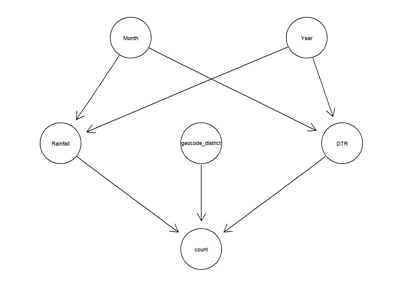
The accuracy of the prediction using Bayesian Network:

##                ME     RMSE      MAE       MPE     MAPE
## Test set 9.386289 22.41716 13.33112 -26.19927 88.27519

The in-sample error is

a <- sqrt(mean((trainCount-pred_train)^2))/sqrt(mean((trainCount)^2))

#for validation data 2013-2015
c <- sqrt(mean((testCount-pred_test)^2))/sqrt(mean((testCount)^2))

The out-sample error for validation data 2013-2015 is

#for validation data 2013-2015
c <- sqrt(mean((testCount-pred_test)^2))/sqrt(mean((testCount)^2))

The mean absolute percentage error:

mape <- function(y, yhat){
  mean(abs((y - yhat)/y), na.rm=T) * 100
}

mpe <- function(y, yhat){
  mean((y - yhat)/y, na.rm=T) * 100
}


mape(testCount, pred_test)

## [1] 88.27519

mpe(testCount, pred_test)

## [1] -26.19927

3.2 Generalized Additive (Mixed) Models

3.2.1 Meterological Data

In this model, the association of meterologiocal variables i.e. DTR and averrage monthly rainfall is considered. I call this Dengue-Meteorological model.

The above summary in Appendix B.2 suggests that all the temperature and rain lag variables are important factors. Let’s visualize the additive model in Figure 3.1.

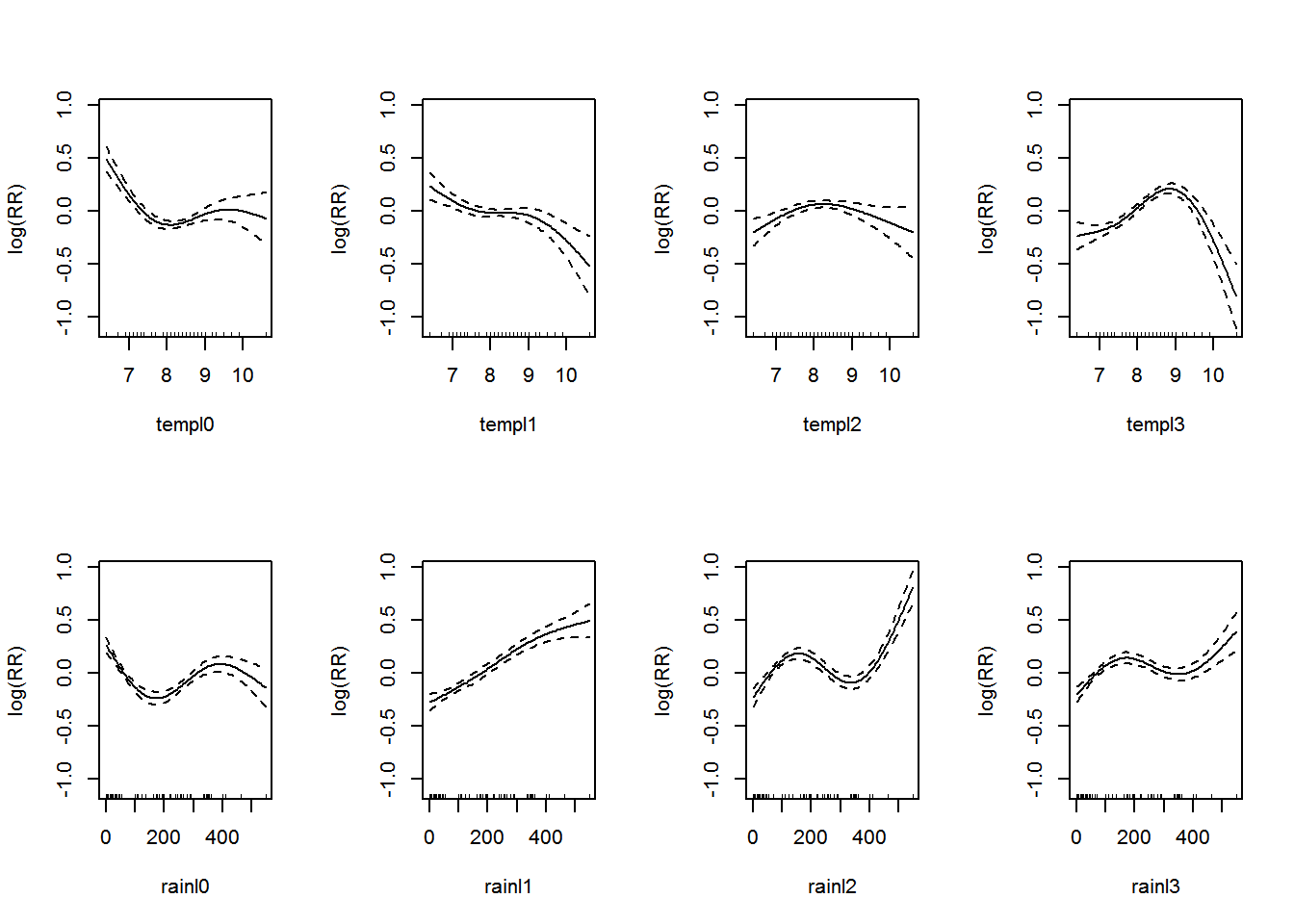
Figure 3.1: Association between the meteorological variables and dengue over lags of 0-3 months.. Solid lines represent relative risks (RR) of dengue cases and dottted lines depict the upper and lower limits of 95% confidence intervals.

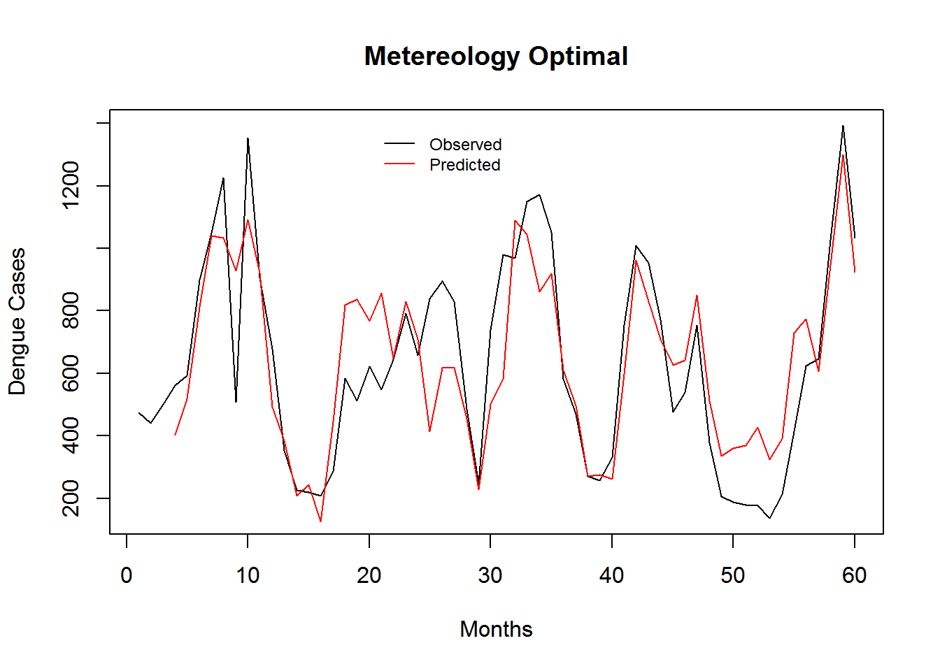
Figure 3.2: Monthly Observed and predicted dengue cases (2008-2012).

Table 3.1: Predictive Performance Statistics of Metereology Model.

Model Name	RMSE	SRMSE	R-sq.(adj)	Deviance Explained
Meteorology Model	8.462372	0.5200771	0.2831722	0.3188542

3.2.2 Dengue Surveillance Data

In this model the association of past denge incidences is considered.

3.2.2.1 Short-term Lag Model

The summary of the model is shown in Appendix B.3. Let’s visualize the additive model in Figure 3.3.

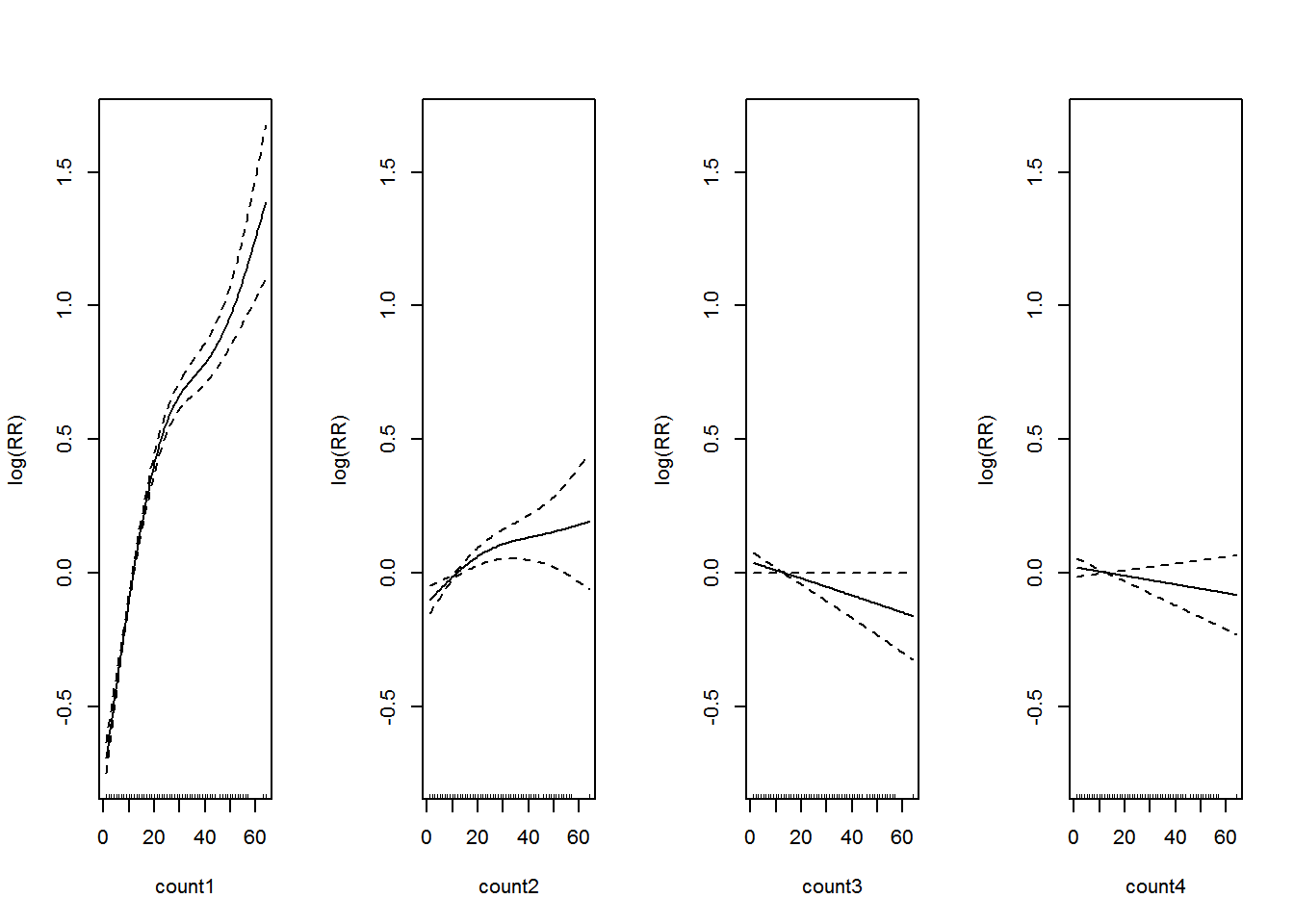
Figure 3.3: Association between past dengue count over lags of 1-4 months and the dengue outbreak.. Solid lines represent relative risks (RR) of dengue cases and dottted lines depict the upper and lower limits of 95% confidence intervals.

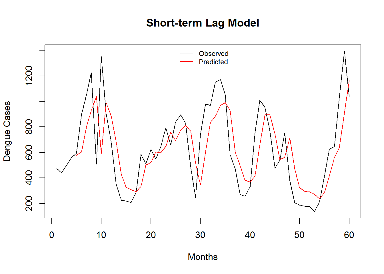
Figure 3.4: Monthly Observed and predicted dengue cases (2008-2012).

Table 3.2: Predictive Performance Statistics of Short-term Lag Model.

Model Name	RMSE	SRMSE	R-sq.(adj)	Deviance Explained
Short-term Lag Model	7.895124	0.4852154	0.3988267	0.4104035

3.2.2.2 Long-term Lag Model

## This is dlnm 2.2.6. For details: help(dlnm) and vignette('dlnmOverview').
## Important changes: see file.show(system.file('Changesince220',package='dlnm'))

I show the simulated lag–response surfaces as relative risk in Figure 3.5.

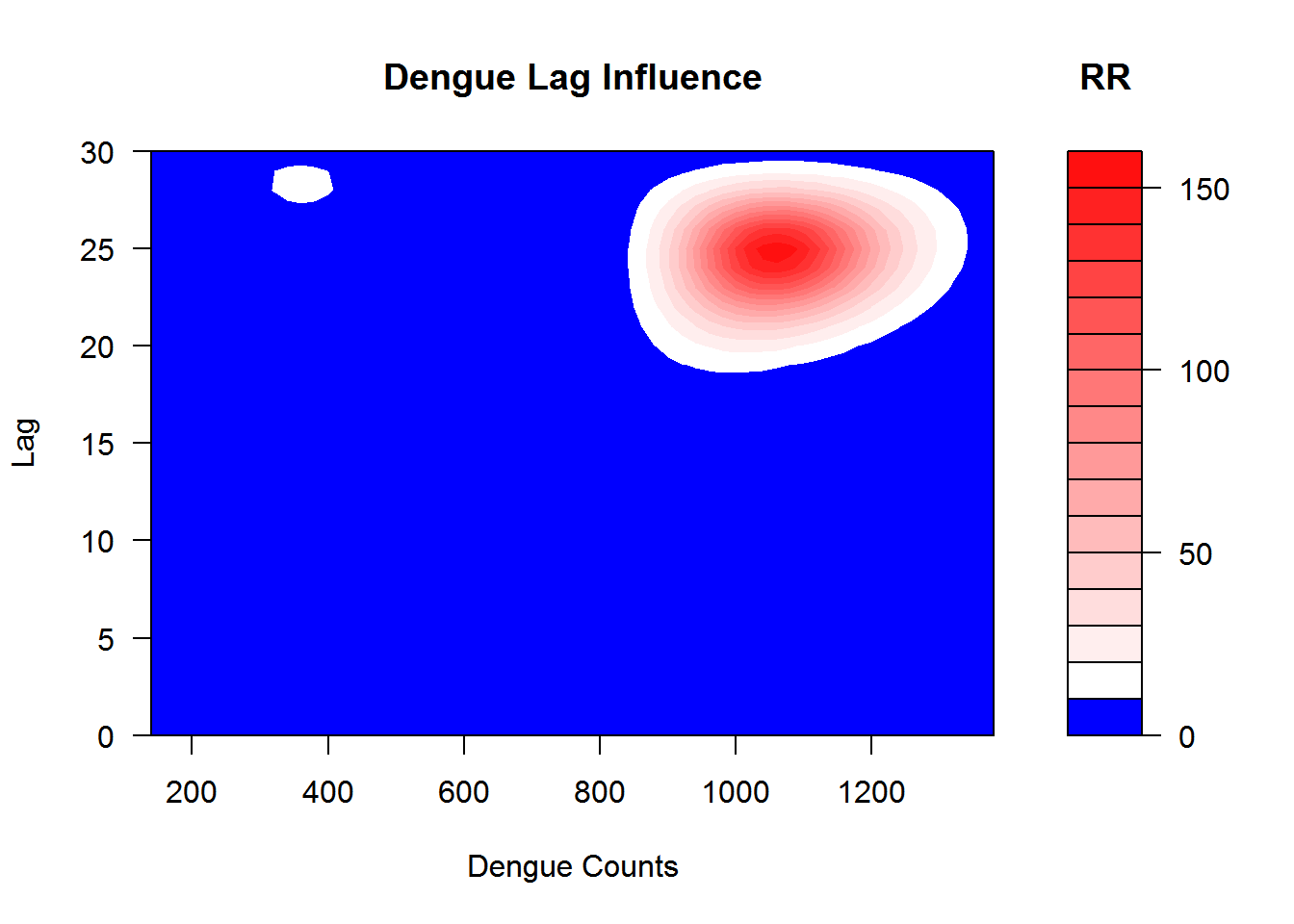
Figure 3.5: This shows the relation between the case intensity and dengue incidences at the lag months

The summary of the model is shown in Appendix B.5. Let’s visualize the additive model in Figure 3.6.

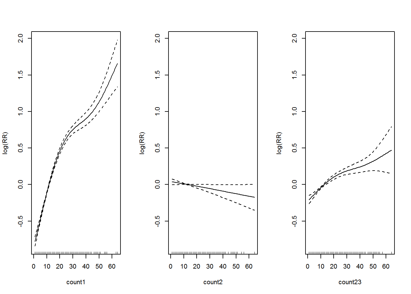
Figure 3.6: Association between past dengue count over optimal lags within 1-30 months and the dengue outbreak.. Solid lines represent relative risks (RR) of dengue cases and dottted lines depict the upper and lower limits of 95% confidence intervals.

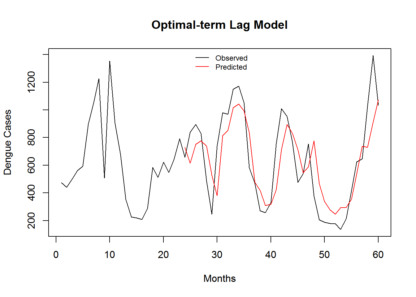
Figure 3.7: Monthly Observed and predicted dengue cases (2008-2012).

Table 3.3: Predictive Performance Statistics of Optimal-term Lag Model.

Model Name	RMSE	SRMSE	R-sq.(adj)	Deviance Explained
Optimal-term Lag Model	7.317273	0.4497021	0.4901485	0.488694

3.2.3 Meteorology and Optimal-term Lag Model.

The summary of the model is shown in Appendix B.6. Let’s visualize the additive model in Figure 3.8.

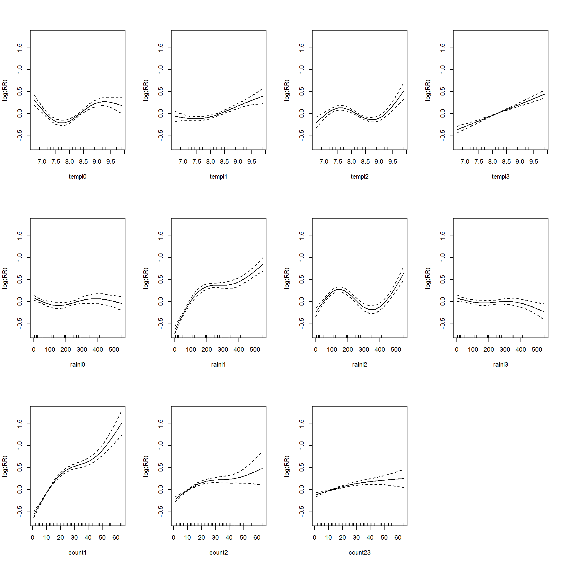
Figure 3.8: Association between the meteorological variables, past dengue count over optimal lags within 1-30 months and the dengue outbreak.. Solid lines represent relative risks (RR) of dengue cases and dottted lines depict the upper and lower limits of 95% confidence intervals.

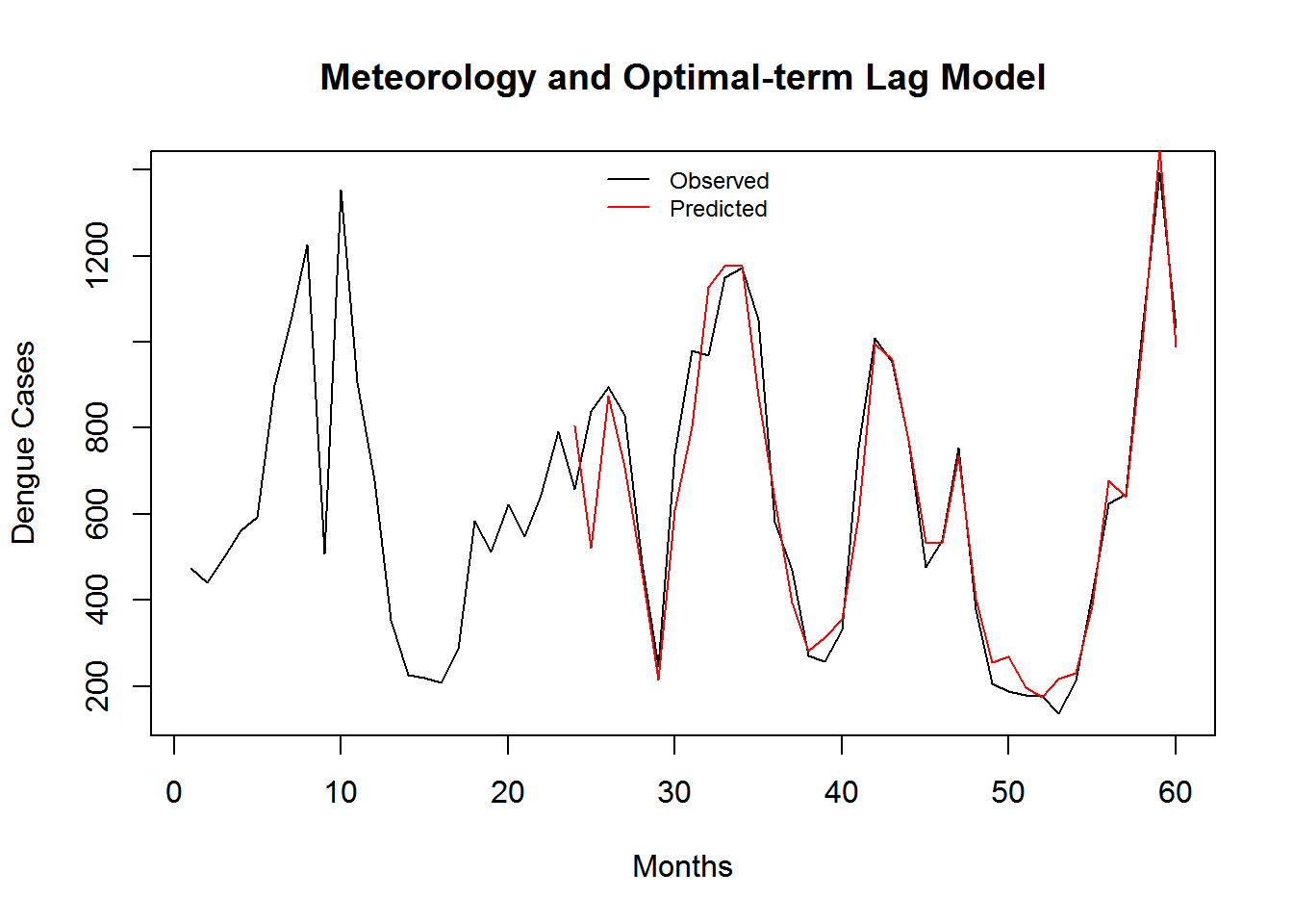
Figure 3.9: Monthly Observed and predicted dengue cases (2008-2012).

Table 3.4: Predictive Performance Statistics of Meteorology and Optimal-term Lag Model.

Model Name	RMSE	SRMSE	R-sq.(adj)	Deviance Explained
Meteorology and Optimal-term Lag Model	6.121665	0.3762228	0.6384466	0.6635623

3.2.4 Surrounding Dengue Data

I show the simulated lag–response surfaces for surrounding districts as relative risk in Figure 3.10.

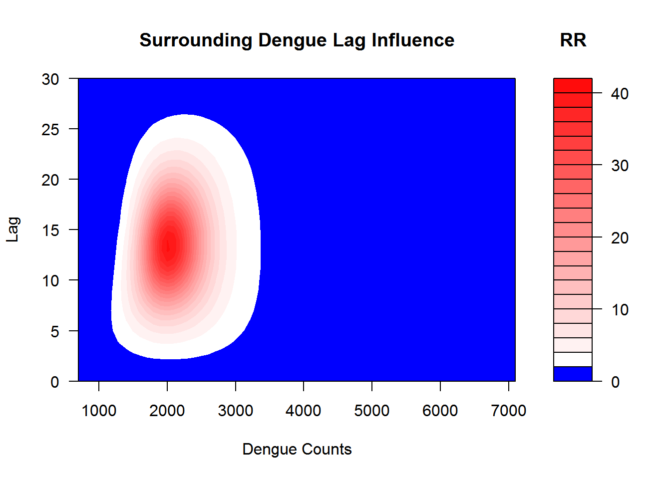
Figure 3.10: This shows the relation between the case intensity and dengue incidences in surrounding districts at the lag months

3.2.5 Meteorology, Optimal-term and Short-term Surrounding Lag Model

The summary of the model is shown in Appendix @ref(appDMDS_Short). Let’s visualize the additive model in Figure @ref(fig:DMDS_Short).

(#fig:DMDS_Short)Association between the meteorological variables, past dengue count over optimal lags within 1-30 months, surroinding district count over 0-3 months and the dengue outbreak.. Solid lines represent relative risks (RR) of dengue cases and dottted lines depict the upper and lower limits of 95% confidence intervals.

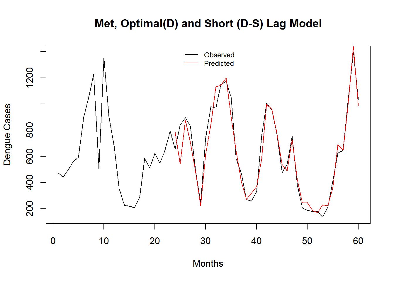
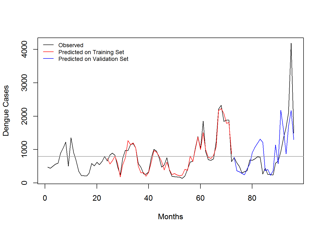
(#fig:DMDSShort_Pred)Monthly Observed and predicted dengue cases (2008-2012).

Table 3.5: Predictive Performance Statistics of Meteorology and Optimal-term Lag Model.

Model Name	RMSE	SRMSE	R-sq.(adj)	Deviance Explained
Meteorology, Optimal(D) Short(D-S) Lag Model	6.000072	0.36875	0.6521614	0.6726038

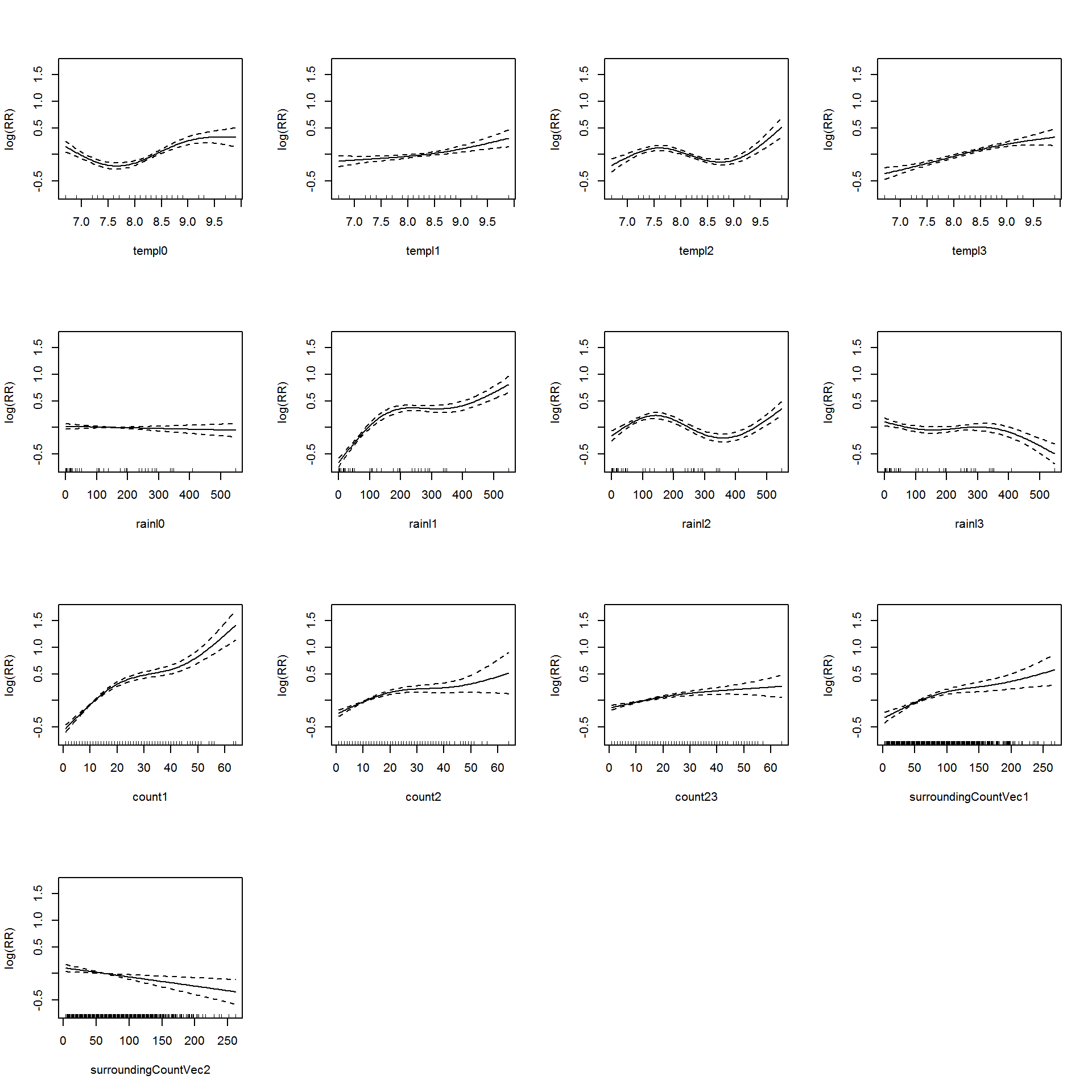
3.2.6 Meteorology, Optimal-term and Optimal-term Surrounding Lag Model

The summary of the model is shown in Appendix @ref(appDMDS_Optimal). Let’s visualize the additive model in Figure @ref(fig:DMDS_Optimal).

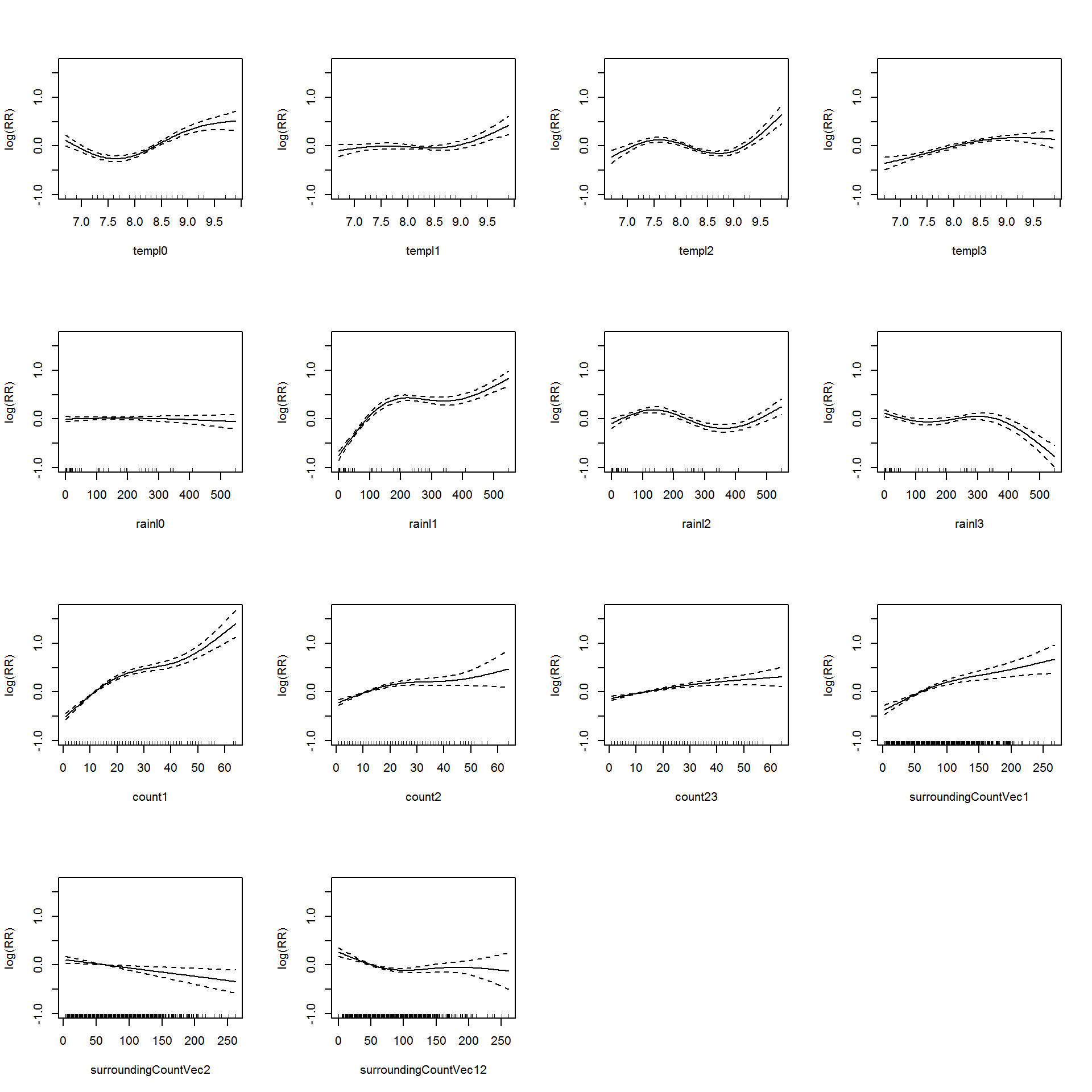
(#fig:DMDS_Optimal)Association between the meteorological variables, past dengue count over optimal lags within 1-30 months, surrounding district count over 0-30 months and the dengue outbreak.. Solid lines represent relative risks (RR) of dengue cases and dottted lines depict the upper and lower limits of 95% confidence intervals.

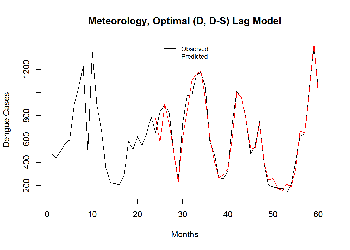
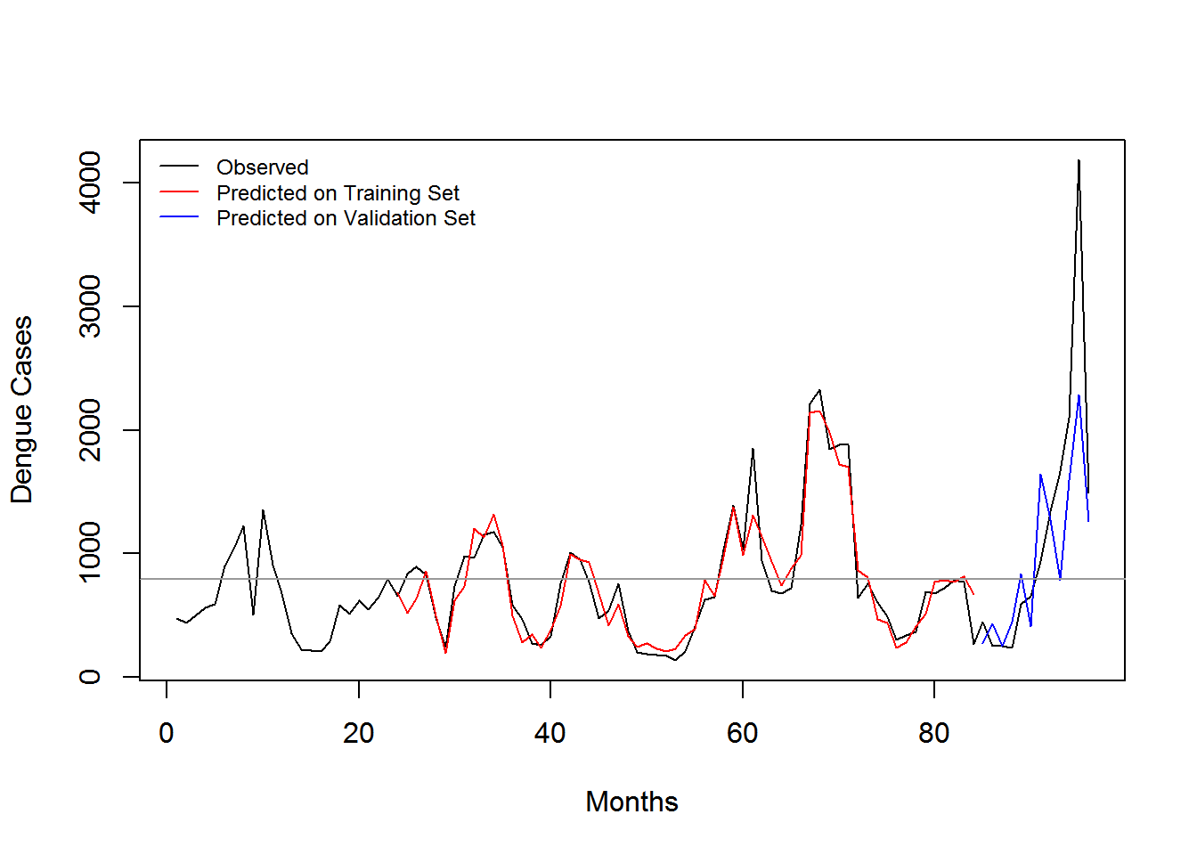
Figure 3.11: Monthly Observed and predicted dengue cases (2008-2012).

Table 3.6: Predictive Performance Statistics of Meteorology and Optimal-term Lag Model.

Model Name	RMSE	SRMSE	R-sq.(adj)	Deviance Explained
Meteorology, Optimal (D, D-S) Lag Model	5.940368	0.3650807	0.6581915	0.6809764

3.3 Social-Economic Data

The summary of the model is shown in Appendix B.9. Let’s visualize the additive model in Figure 3.12.

Figure 3.12: Association between the meteorological variables, past dengue count over optimal lags within 1-30 months, surrounding district count over 0-30 months, garbage data and the dengue outbreak.. Solid lines represent relative risks (RR) of dengue cases and dottted lines depict the upper and lower limits of 95% confidence intervals.

Figure 3.13: Monthly Observed and predicted dengue cases (2008-2012).

Table 3.7: Predictive Performance Statistics of Social-economic data Included.

Model Name	RMSE	SRMSE	R-sq.(adj)	Deviance Explained
Social-economic data Included	5.924147	0.3640839	0.6594216	0.7457561

3.4 Predictive Performance Statistics

On the training dataset.

Table 3.8: Predictive Performance Statistics of All Models

Model Name	RMSE	SRMSE	R-sq.(adj)	Deviance Explained
Meteorology Model	8.462372	0.5200771	0.2831722	0.3188542
Short-term Lag Model	7.895124	0.4852154	0.3988267	0.4104035
Optimal-term Lag Model	7.317273	0.4497021	0.4901485	0.4886940
Meteorology and Optimal-term Lag Model	6.121665	0.3762228	0.6384466	0.6635623
Meteorology, Optimal(D) Short(D-S) Lag Model	6.000072	0.3687500	0.6521614	0.6726038
Meteorology, Optimal (D, D-S) Lag Model	5.940368	0.3650807	0.6581915	0.6809764
Social-economic data Included	5.924147	0.3640839	0.6594216	0.7457561

3.5 Evaluation

Table 3.9: Predictive Performance Statistics measured using SRMSE

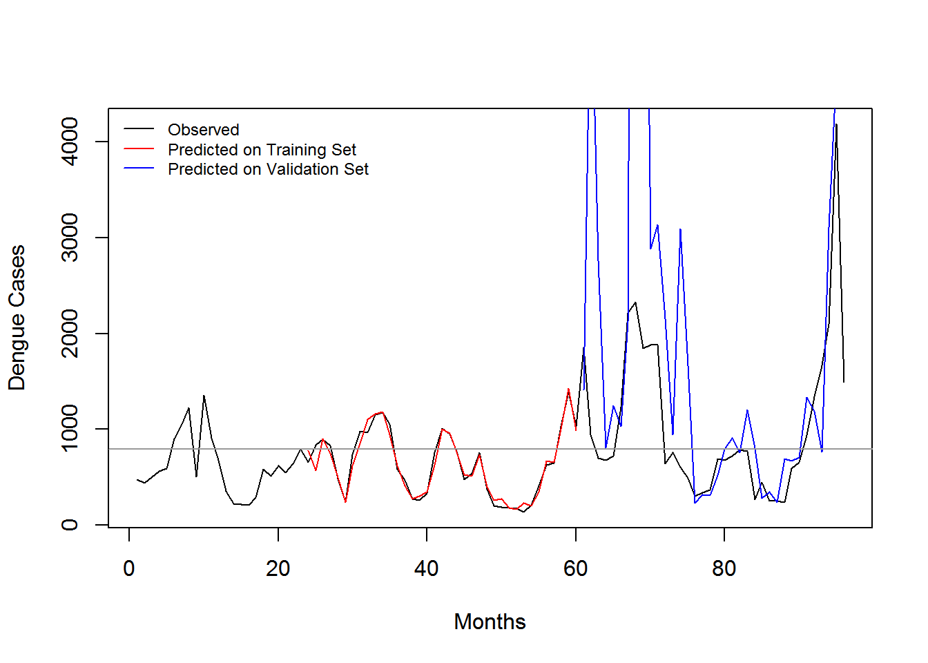
Training Dataset	In-sample Error	Out-Sample (2013-2015)	Out-Sample (2014-2015)	Out-Sample (2013)	Out-Sample (2014)	Out-Sample (2015)
2008-2012	0.3650807	303.282	410.7401247	21.66415	1.4334466	437.4985502
2008-2013	0.3843044	NA	0.5627701	NA	0.3202835	0.5354210
2008-2014	0.3940100	NA	NA	NA	NA	0.4888606