8 Lab 8: Systematic Conservation Planning
library(prioritizr) # Our new package for SCP
library(prioritizrdata) # Case study data from Hanson et al. 2025 Conservation Biology
#library(gurobi) # This is a generally recommended solver but not available for R 4.4.3...
library(highs) # Import a different solver; this may be slower than Gurobi but is available
library(sf)
library(raster)
library(ggplot2)
library(terra)
library(tidyverse)
library(rnaturalearth) # For state shapefiles preloaded
8.1 Some Pre-Processed Data You May Find Helpful:
Note: Feel free to delete all this if you aren’t using it for your submission to save on runtime.
LAND VALUES: A useful dataset may be the PLACES dataset which has private property values estimated across the US. Values are USD per hectare logged (natural log).
# Read the GeoTIFF file PLACES land value for the US
land_value_raster <- rast("places_fmv_vacant.tif")
plot(land_value_raster)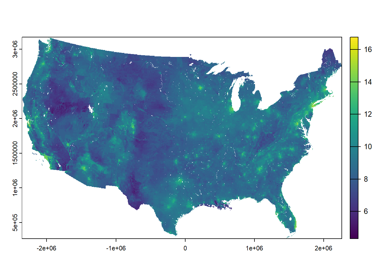
Bring in Michigan Shapefile to trim to:
# Get Michigan shape
michigan_boundary <- ne_states(returnclass = "sf") %>%
  filter(name == "Michigan")

# Reproject to NAD83 CONUS Albers like PLACES
michigan_boundary <- st_transform(michigan_boundary, crs = "EPSG:5070")
Crop and plot PLACES to Michigan only
# Crop to MI
land_value_raster_cropped <- crop(land_value_raster, michigan_boundary)

# Mask to remove non-MI
land_value_raster_masked <- mask(land_value_raster_cropped, michigan_boundary)

MI_land_dollars <-exp(land_value_raster_masked)

# Plot just MI PLACES values
plot(MI_land_dollars, main = "Vacant land value MI $/ha")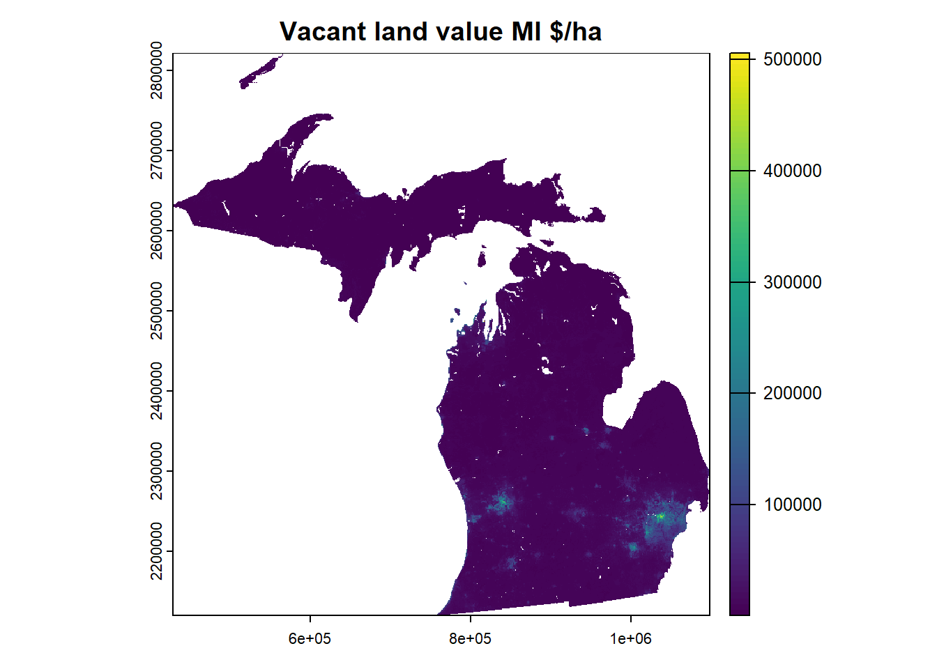
PROTECTED AREAS: This is a file I preprocessed at the same resolution/scale as the PLACES dataset above using a subset of the PAD-US dataset (Forest Service designated areas). Note that this is not the full PAD-US dataset and I created this for simplicity for this exercise.
Read in PADUS FS raster
Again, crop to MI as above as an example to create two potential rasters for a stack. You may use a different MI, a different state, extent, or none of this.
# Crop to MI
padus_raster_cropped <- crop(padus, michigan_boundary)

# Mask to remove non-MI
padus_raster_masked <- mask(padus_raster_cropped, michigan_boundary)

# Plot just MI PLACES values
plot(padus_raster_masked, main = "MI PADUS - Forest Service Designated Areas")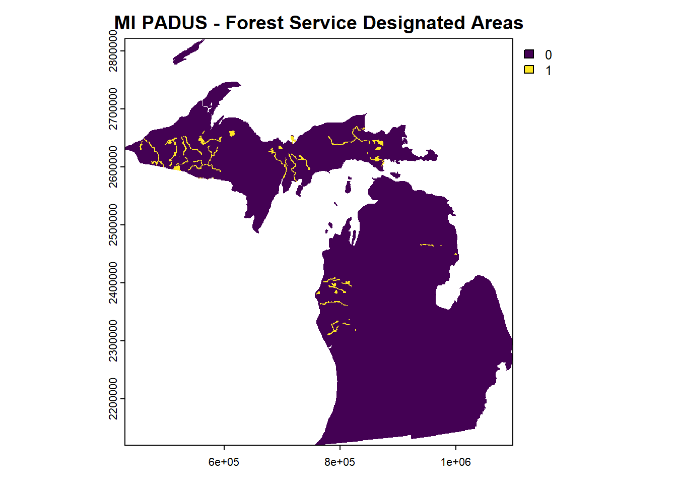
8.2 Part 1: Specifying you optimization problem (30 pts)
- Describe your optimization problem, including the descriptions of your PUs, features, targets, objective, constraints, and penalties (5 pts each):
Recall for our WA state example, the features were the bird distribution maps, the targets were 20% coverage of each bird map, the objective was to best satisfy the targets for a specific budget. The extended example included lock and lock out constraints based on already protected areas and urban areas, as well as a boundary penalty.
Your own optimization problem does not need to be conservation-based, but the more railroaded exercise here can use the above two rasters plus some other data for your targets.
8.3 Part 2: Import and harmonize your data (20 pts)
As with many of our functions, you will need to preprocess your data to the same extent and (often) resolution prior to running. The most straightforward way to do this process for prioritzr is to only use rasters that all have the identical spatial extent, resolution, and CRS.
- You may process your data however you please, and grading will be based on showing the target raster (10 pts) and the cost/objective raster (10 pts). If your target is a large raster stack like in the WA state birds just show a small slice of the stack.
8.4 Part 3: Specify your SDM/Problem (30 pts)
- Next, set up a “problem” with your PUs, features, targets, objective, constraints, and penalties from Part 1. In the problem, please annotate which line is each part of your problem (5 pts each):
8.5 Part 4: Solve your Problem (20 pts)
Next, you will solve your problem. For the sake of this exercise, please feel free to use an excessive gap like 25% so that it runs faster (10 pts).
Assess some component of your optimal (or near-optimal) solution such as how well targets are being met. Please do this numerically with code (5 pts) as well as write a few sentence interpretation (5 pts)