5 Lab 7 Intro
5.1 Introduction
Classification is a common task in ecology both at our landscape scales analyses and at other biological scales. We often don’t have cleanly designed experiments in ecology and datasets often suffer from class imbalance, where some class that we are trying to identify (species ID, land use type, community state, etc.) are overrepresented. In this lab, we will use the CPU core scalable Random Forest (ranger) package to for a multiclass (3+) classification problem. For your own exercise, you can choose any ecological dataset including the forest inventory one I have prepared and explore random forest models addressing class imbalance and optimizing model hyperparameters.
library(ranger)       # Multicore random forest (+ more advanced tuning)
library(palmerpenguins)      # Penguin dataset for my worked example
library(caret)        # Tuning and cross-validation
library(ggplot2)
library(dplyr)
library(tibble)     # Wrangling for
library(yardstick)    # Model evaluation metrics - boring name
library(tune)         # Hyperparameter tuning
library(workflowsets) # Machine learning workflows
library(parsnip)      # Unified ML interface - fun name
library(pdp)             # Makes partial dependence plots for the random forests
library(tidyr)
First, I will bring in an imbalanced dataset of penguin species
# Load dataset and remove missing values
df <- na.omit(penguins) # This removes any rows with missing data, you may have to be more selective with personal data

# Convert species to a factor (classification target variable) - essential step!
df$species <- as.factor(df$species)

# Split into training (80%) and test (20%) sets, similar to our SDM exercise
set.seed(42)
trainIndex <- createDataPartition(df$species, p = 0.8, list = FALSE)
train_df <- df[trainIndex, ]
test_df <- df[-trainIndex, ]

# Check class distribution
table(train_df$species)
##
## Adelie Chinstrap Gentoo
## 117 55 96# Plot class imbalance
ggplot(train_df, aes(x = species)) +
geom_bar(fill = "lightblue") +
theme_minimal() +
labs(title = "Class Imbalance in Palmer Penguins Training Dataset", x = "Species", y = "Count")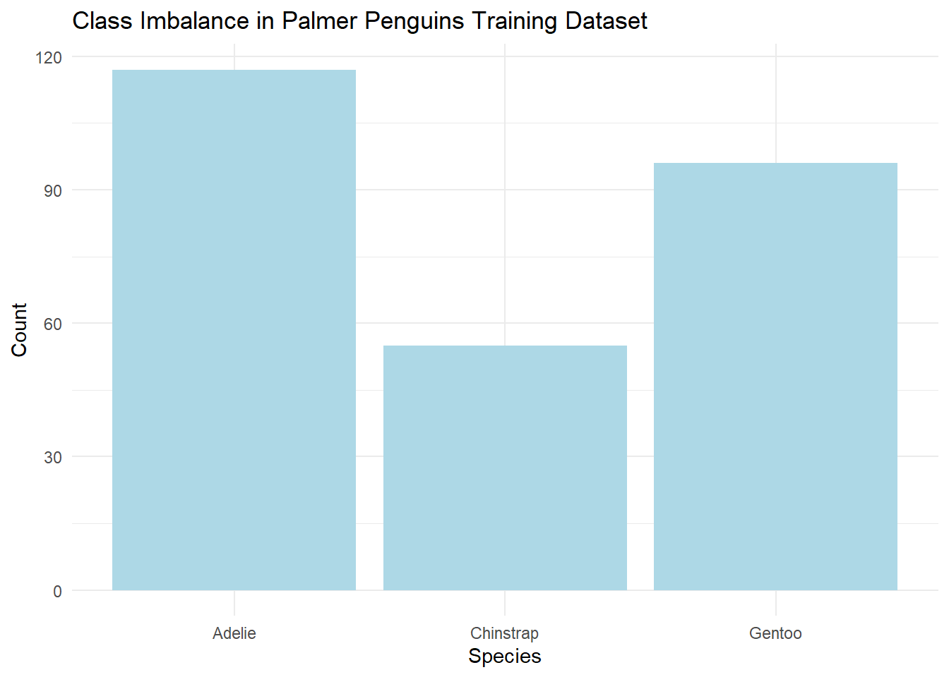
Our goal is to classify the penguins based on theirr bills, flippers, bodymass, sex, and location:
## # A tibble: 6 × 8
##   species island    bill_length_mm bill_depth_mm flipper_length_mm body_mass_g
##   <fct>   <fct>              <dbl>         <dbl>             <int>       <int>
## 1 Adelie  Torgersen           39.1          18.7               181        3750
## 2 Adelie  Torgersen           39.5          17.4               186        3800
## 3 Adelie  Torgersen           40.3          18                 195        3250
## 4 Adelie  Torgersen           36.7          19.3               193        3450
## 5 Adelie  Torgersen           39.3          20.6               190        3650
## 6 Adelie  Torgersen           38.9          17.8               181        3625
## # ℹ 2 more variables: sex <fct>, year <int>
5.2 Random forest in ranger
First, let’s try a base random forest to classify the penguins. Here we will use the defaults without any tuning or weighting for class imbalances. We will use 500 trees which is also the default for randomForest, as I recall:
# Train a baseline Random Forest model
baseline_rf <- ranger(
  species ~ ., # The . says to use all other columns in the data, you may need to specify a subset for your own work
  data = train_df,
  num.trees = 500,
  importance = "impurity",
  probability = TRUE,
  num.threads = 4 # Scale the analysis to 4 cores
)

# Predict on test set (Extract class labels from probability matrix)
baseline_pred_matrix <- predict(baseline_rf, test_df)$predictions
baseline_preds <- apply(baseline_pred_matrix, 1, function(x) names(which.max(x)))
baseline_preds <- factor(baseline_preds, levels = levels(test_df$species))

# Compute Balanced Accuracy
test_results <- tibble(truth = test_df$species, predicted = baseline_preds) # This will also work with data.frame if you like
balanced_acc_baseline <- bal_accuracy(test_results, truth, predicted)
print(balanced_acc_baseline)
## # A tibble: 1 × 3
## .metric .estimator .estimate
## <chr> <chr> <dbl>
## 1 bal_accuracy macro 0.9745.2.1 Random forest with class weights
We can also specify a class weights argument. There are a variety of ways in which imbalance can be addressed in a random forest, but in this case it’s increasing how important it views the minimization of errors inversely proportionally to the number of penguins of a species. I.e., I am telling it that I want it to care a bit more about chinstrap penguin error than for the other two species.
# Compute inverse frequency class weights
class_counts <- table(train_df$species)
class_weights <- 1 / class_counts
class_weights <- class_weights / sum(class_weights) # Normalize weights

# Train a weighted Random Forest model
weighted_rf <- ranger(
  species ~ .,
  data = train_df,
  num.trees = 500,
  class.weights = class_weights,
  probability = TRUE,
  num.threads = 4 # Scale the analysis to 4 cores
)

# Predict on test set (Extract class labels)
weighted_pred_matrix <- predict(weighted_rf, test_df)$predictions
weighted_preds <- apply(weighted_pred_matrix, 1, function(x) names(which.max(x)))
weighted_preds <- factor(weighted_preds, levels = levels(test_df$species))

# Compute Balanced Accuracy
test_results <- tibble(truth = test_df$species, predicted = weighted_preds)
balanced_acc_weighted <- bal_accuracy(test_results, truth, predicted)
print(balanced_acc_weighted)
## # A tibble: 1 × 3
## .metric .estimator .estimate
## <chr> <chr> <dbl>
## 1 bal_accuracy macro 0.9745.2.2 Random forest with search grid
Next, we can tune the model hyperparameters by creating a search grid to find the combination of tree building parameters and number of trees that optimize our outcome (balanced accuracy). There are a few other hyperparameters you may want to consider as well, but these three are some of the major ones.
# Define parameter grid
grid <- expand.grid(
  num.trees = c(500, 1000),
  mtry = floor(sqrt(ncol(train_df) - 1)),
  min.node.size = c(1, 5, 10)
)

# Perform grid search
grid_results <- lapply(1:nrow(grid), function(i) {
  rf <- ranger(
    species ~ .,
    data = train_df,
    num.trees = grid$num.trees[i],
    mtry = grid$mtry[i],
    min.node.size = grid$min.node.size[i],
    probability = TRUE,
    num.threads = 4 # Scale the analysis to 4 cores
  )
  preds <- predict(rf, test_df)$predictions
  preds <- apply(preds, 1, function(x) names(which.max(x)))
  preds <- factor(preds, levels = levels(test_df$species))

  test_results <- tibble(truth = test_df$species, predicted = preds)
  balanced_acc <- bal_accuracy(test_results, truth, predicted)

  return(data.frame(
    num.trees = grid$num.trees[i],
    mtry = grid$mtry[i],
    min.node.size = grid$min.node.size[i],
    balanced_acc = balanced_acc$.estimate
  ))
})

# Convert results to a data frame and select best model
grid_results_df <- do.call(rbind, grid_results)
best_grid_model <- grid_results_df %>% arrange(desc(balanced_acc)) %>% head(1)
grid_results_df # You may not want to print this if you did a giant search grid
## num.trees mtry min.node.size balanced_acc
## 1 500 2 1 0.9825499
## 2 1000 2 1 0.9825499
## 3 500 2 5 0.9735976
## 4 1000 2 5 0.9825499
## 5 500 2 10 0.9735976
## 6 1000 2 10 0.9735976## num.trees mtry min.node.size balanced_acc
## 1 500 2 1 0.98254995.2.3 Random forest with random search
If we have a bigger range of hyperparameter space we need to explore and don’t have the ability to fully explore as in a grid search, we can also explore using a random search. We still need to create a dataframe as before to define our total search space, but this time we randomly samply combinations within the search space, choosing the best one.
set.seed(42) # Note we should set a seed since we are doing something random!!
random_search <- data.frame(
  num.trees = sample(seq(500, 1500, by = 50), 4),
  mtry = sample(2:5, 4),
  min.node.size = sample(c(1:15), 4)
)

# Perform random search
random_results <- lapply(1:nrow(random_search), function(i) {
  rf <- ranger(
    species ~ .,
    data = train_df,
    num.trees = random_search$num.trees[i],
    mtry = random_search$mtry[i],
    min.node.size = random_search$min.node.size[i],
    probability = TRUE,
    num.threads = 4 # Scale the analysis to 4 cores
  )
  preds <- predict(rf, test_df)$predictions
  preds <- apply(preds, 1, function(x) names(which.max(x)))
  preds <- factor(preds, levels = levels(test_df$species))

  test_results <- tibble(truth = test_df$species, predicted = preds)
  balanced_acc <- bal_accuracy(test_results, truth, predicted)

  return(data.frame(
    num.trees = random_search$num.trees[i],
    mtry = random_search$mtry[i],
    min.node.size = random_search$min.node.size[i],
    balanced_acc = balanced_acc$.estimate
  ))
})

# Convert results to a data frame and select best model
random_results_df <- do.call(rbind, random_results)
best_random_model <- random_results_df %>% arrange(desc(balanced_acc)) %>% head(1)
print(best_random_model)
## num.trees mtry min.node.size balanced_acc
## 1 950 2 4 0.98254995.2.4 Variable importance for best model
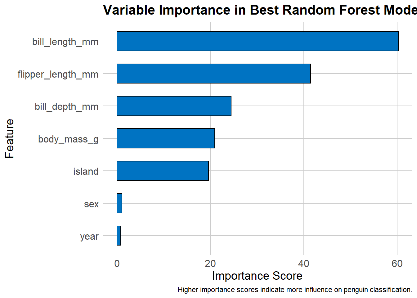
For your own exercise, you don’t need to identify the best model across all methods, just within either one grid search or one random search. As before, we can display the variable importance from our random forest model.
# Train the best random model
final_model <- ranger(
  species ~ .,
  data = train_df,
  num.trees = best_random_model$num.trees,
  mtry = best_random_model$mtry,
  min.node.size = best_random_model$min.node.size,
  importance = "impurity",
  probability = TRUE,
  num.threads = 4 # Scale the analysis to 4 cores
)

importance_df <- as.data.frame(final_model$variable.importance) %>%
  tibble::rownames_to_column("Feature") %>%
arrange(desc("final_model$variable.importance"))ggplot(importance_df, aes(x = reorder(Feature, final_model$variable.importance), y = final_model$variable.importance)) +
geom_bar(stat = "identity", fill = "#0073C2", color = "black", width = 0.6) +
theme_minimal() +
coord_flip() +
labs(
title = "Variable Importance in Best Random Forest Model",
x = "Feature",
y = "Importance Score",
caption = "Higher importance scores indicate more influence on penguin classification."
) +
theme(
plot.title = element_text(size = 16, face = "bold"),
axis.text = element_text(size = 12),
axis.title = element_text(size = 14),
panel.grid.major = element_line(color = "gray80"),
panel.grid.minor = element_blank()
)
5.2.5 Partial dependence plots
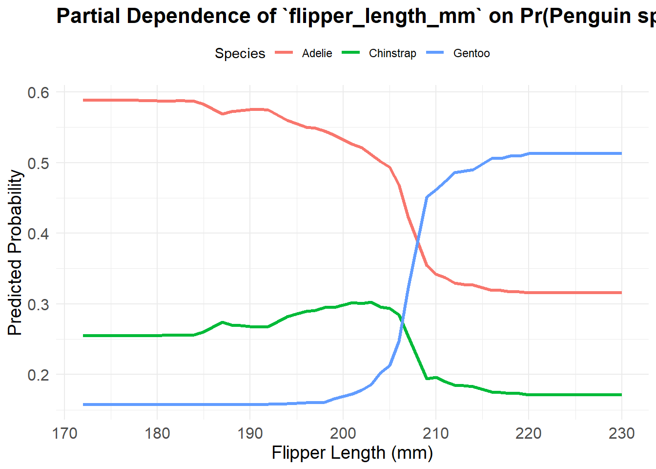
One of the main ways to make output from a random forest interpretable to us end users is to use a partial dependence plot. Essentially, these are the ML predictions when setting all other variables constant - we do similar things in prediction output from linear models as well. These can be incredibly computationally costly to create, even much more so than the random forest models themselves. I wouldn’t suggest creating one for your own exercise unless your data are relatively small and straightforward.
# Extract species levels
species_levels <- levels(train_df$species)

# Compute partial dependence separately for each species
pdp_list <- lapply(species_levels, function(sp) {
  pd <- partial(
    object = final_model,          # Best trained Random Forest model
    pred.var = "flipper_length_mm", # Feature to analyze
    train = train_df,              # Training dataset
    which.class = sp,              # Compute for one species at a time
    prob = TRUE                    # Get class probabilities
  )

  # Convert to data frame and add species label
  pd_df <- as.data.frame(pd)
  pd_df$Species <- sp

  return(pd_df)
})

# Combine all species-specific partial dependence data
pdp_df <- bind_rows(pdp_list)ggplot(pdp_df, aes(x = flipper_length_mm, y = yhat, color = Species)) +
geom_line(size = 1.2) +
theme_minimal() +
labs(
title = "Partial Dependence of `flipper_length_mm` on Pr(Penguin spp.)",
x = "Flipper Length (mm)",
y = "Predicted Probability",
color = "Species"
) +
theme(
plot.title = element_text(size = 16, face = "bold"),
axis.text = element_text(size = 12),
axis.title = element_text(size = 14),
legend.position = "top"
)
5.3 FIA Data
For your portion of the lab, I have created some Forest Inventory and Analysis data alongside elevation, soil, and MODIS satellite information that you may use. These data are for ~4500 FIA plots across states in the Great Lakes basin for a single sample in 2013 that I matched up with median 2013 MODIS Surface Reflectance bands, elevation data, and then just a handful of SoilGrids data. Unfortunately this process was so slow in R that I had to execute it in Google Earth Engine.
##   FORTYPCD GROWTH_HABIT_CD LAND_COVER_CLASS_CD   SR_B1   SR_B2   SR_B3   SR_B4
## 1      101              FB                   1  8519.5  8994.0 10471.0  9655.5
## 2      102              FB                   1  8141.5  8343.5  9392.0  8862.0
## 3      102              FB                   1  7732.0  7873.0  9724.0  9553.0
## 4      102              FB                   1 24655.0 24087.0 23379.0 23203.0
## 5      102              FB                   1  8636.0  9210.5 11276.5 11122.0
## 6      102              FB                   1  7825.5  7983.5  8741.5  8354.5
##     SR_B5   SR_B6   SR_B7 elevation soil_organic_carbon soil_pH soil_texture
## 1 17818.0 12038.0 10167.0       378                   8      51            9
## 2 18710.5 12201.5 10274.5       238                   6      54            9
## 3 18499.0 12318.0 10307.0       391                  13      56            9
## 4 26110.0 14852.0 12226.0       239                  18      59            9
## 5 19641.5 12777.0 11811.5       236                  14      50            9
## 6 15765.5 11002.0  9246.0       230                  26      50            9
The variables here are the following. Note that particularly the forest type code will be tricky since it has many classes and may need some preprocessing for exceptionally rare classes such as ones with only 1 record.
Variable Descriptions:
| Variable | Description |
|---|---|
FORTYPCD |
Forest type code from FIA |
GROWTH_HABIT_CD |
Growth habit classification from FIA |
LAND_COVER_CLASS_CD |
Land cover classification from FIA |
SR_B1 |
MODIS Surface Reflectance Band 1 |
SR_B2 |
MODIS Surface Reflectance Band 2 |
SR_B3 |
MODIS Surface Reflectance Band 3 |
SR_B4 |
MODIS Surface Reflectance Band 4 |
SR_B5 |
MODIS Surface Reflectance Band 5 |
SR_B6 |
MODIS Surface Reflectance Band 6 |
SR_B7 |
MODIS Surface Reflectance Band 7 |
elevation |
Digital Elevation Model (DEM) elevation in meters |
soil_organic_carbon |
Soil organic carbon content from SoilGrids |
soil_pH |
Soil pH from SoilGrids |
soil_texture |
Soil texture classification from SoilGrids |
5.4 sparklyr
You may also practice setting up an Apache Spark R session and run a distributed random forest without any hyperparameter tuning for your exercise. You will want to go through a more extended guide since there’s a lot of considerations the cannot be covered in a short format as in this class. The installation and setup, and getting all of the components Spark, Java, Hadoop versions, etc all set up properly can be quite frustrating and I’d likely end up having to troubleshoot everyone’s computer individually to get it all working. It all looks (and once set up is) simple, which is why it’s so powerful, but you may spend more time setting this up than using ranger.
But, essentially, to get started you first need to install a version of Spark.
#library(sparklyr)
#spark_install("3.5") # You would do this one time like in our install of the PDF compiler
You would then initiate a Spark session, either locally for testing or connect to a cluster. This is a local version.
It should automatically do the newest version, you can also set up the number of virtual “workers” even on your local machine:
Once you open the Spark connection, you will be able to use Spark dataframes which can be used in a distributed fashion as well as use distributed versions of machine learning (other other) functions such as ml_random_forest. As always, each function is specified slightly differently but it’s still in this case a classification random forest, this time just for the Gentoo class:
# Filter for Gentoo Penguins and convert species column to binary (Gentoo = 1, others = 0)**
#penguins_df <- na.omit(penguins)
#penguins_df <- penguins_df %>%
#  mutate(gentoo = ifelse(species == "Gentoo", 1, 0)) %>%
#  select(-species)  # Remove original species column

# Copy data to a Spark dataframe
#penguins_tbl <- sdf_copy_to(sc, penguins_df, "penguins_spark", overwrite = TRUE)

# Train a Basic Random Forest Model in Spark
#spark_model <- penguins_tbl %>%
#  ml_random_forest(
#    response = "gentoo",   # Predicting Gentoo presence
#    features = c("bill_length_mm", "bill_depth_mm", "flipper_length_mm", "body_mass_g"),  # Feature variables
#    type = "classification"
#  )

#spark_model


# Disconnect from Spark!!!!
#spark_disconnect(sc)
Make sure to disconnect when you are done since otherwise you will still have local resources allocated to Spark workers or be using remote clusters (they probably will boot you after 1-2 hrs but still). If you would like to practice with a remote cluster, Databricks has a free Community Edition that you can sign up for that will let you create and connect to a compute that is about the size of an average computer just to explore.