7 Lab 8 SCP Tutorial
7.1 SCP & Optimization
Systematic conservation planning (SCP) is a structured approach to designing protected areas and managing landscapes for biodiversity conservation. It is an optimization problem where we want to maximize conservation benefits (targets) while minimizing costs (our objective).
Optimization problems are in no way restricted to SCP, but I thought that this would be a nice ending lab since it can use many of the inputs from our previous exercises such as our MaxEnt output. It also is a way to add a management/human/practical component that we haven’t had much of yet. That said, optimization as a general method is something else to keep in your toolbox even if you aren’t focused on conservation planning as many other problems are should be treated in this manner. For example, even something like choosing sampling sites for an experiment may be a tough optimization problem to balance accessibility, driving distance, areas that you need to lock in/lock out, and be something you can’t solve simply.
We will focus on using the prioritizr R package, which is a handy wrapper for the optimization process using spatial data. Like so many of our previous analyses, the major input is the stack of rasters - in this case those relevant to your targets, objectives, and constraints to solve for.
library(prioritizr) # Our new package for SCP
library(prioritizrdata) # Case study data from Hanson et al. 2025 Conservation Biology
#library(gurobi) # This is a generally recommended solver but not available for R 4.4.3...
library(highs) # Import a different solver; this may be slower than Gurobi but is available
library(sf)
library(raster)
library(ggplot2)
library(terra)
library(tidyverse)
7.2 Example SCP
We will use the case study from Hanson et al. 2025, Conservation Biology. The case study applies systematic conservation planning to Washington State.
An SCP uses some optimization algorithm to identify areas to prioritize (for management, preservation, or something else). Some SCP methods use iterative algorithms like Marxan we discussed in class on Tuesday, which may or may not get to THE optimal mathematical solution. I am choosing to introduce prioritizr since I think its feature of having an exact solution solver more generally applicable to other problems. Note: you actually may set a “gap” in prioritizr so that it provides a solution 5%, 10%, etc away from the optimum. There are multiple solvers in prioritizr, and it will automatically select the “best”.
The overall SCP here looked at conservation lands in Washington State valued at $3013.56 million with the goal of increasing the conservation land value by 30% to $3917.63 million). The conservation target was birds in the state with the input being 396 species distribution maps for 258 bird species (applying multiple maps for seasonality). Since this study was performed by the authors of R package, they have conveniently made the data available through the R data package prioritizrdata.
7.2.1 Step 1: Planning Units
The first step is to identify the Planning Units (PUs) that the conservation problem is being applied to. As with many things in landscape ecology, the default unit is often our raster grid cell but note that the package can also be applied to shapefile data (as sf polygons) as well.
# import planning unit data from Hanson et al. 2025
wa_pu <- get_wa_pu()

# preview data
print(wa_pu)
## class : SpatRaster
## dimensions : 109, 147, 1 (nrow, ncol, nlyr)
## resolution : 4000, 4000 (x, y)
## extent : -1816382, -1228382, 247483.5, 683483.5 (xmin, xmax, ymin, ymax)
## coord. ref. : +proj=laea +lat_0=45 +lon_0=-100 +x_0=0 +y_0=0 +ellps=sphere +units=m +no_defs
## source : wa_pu.tif
## name : cost
## min value : 0.2986647
## max value : 1804.1838379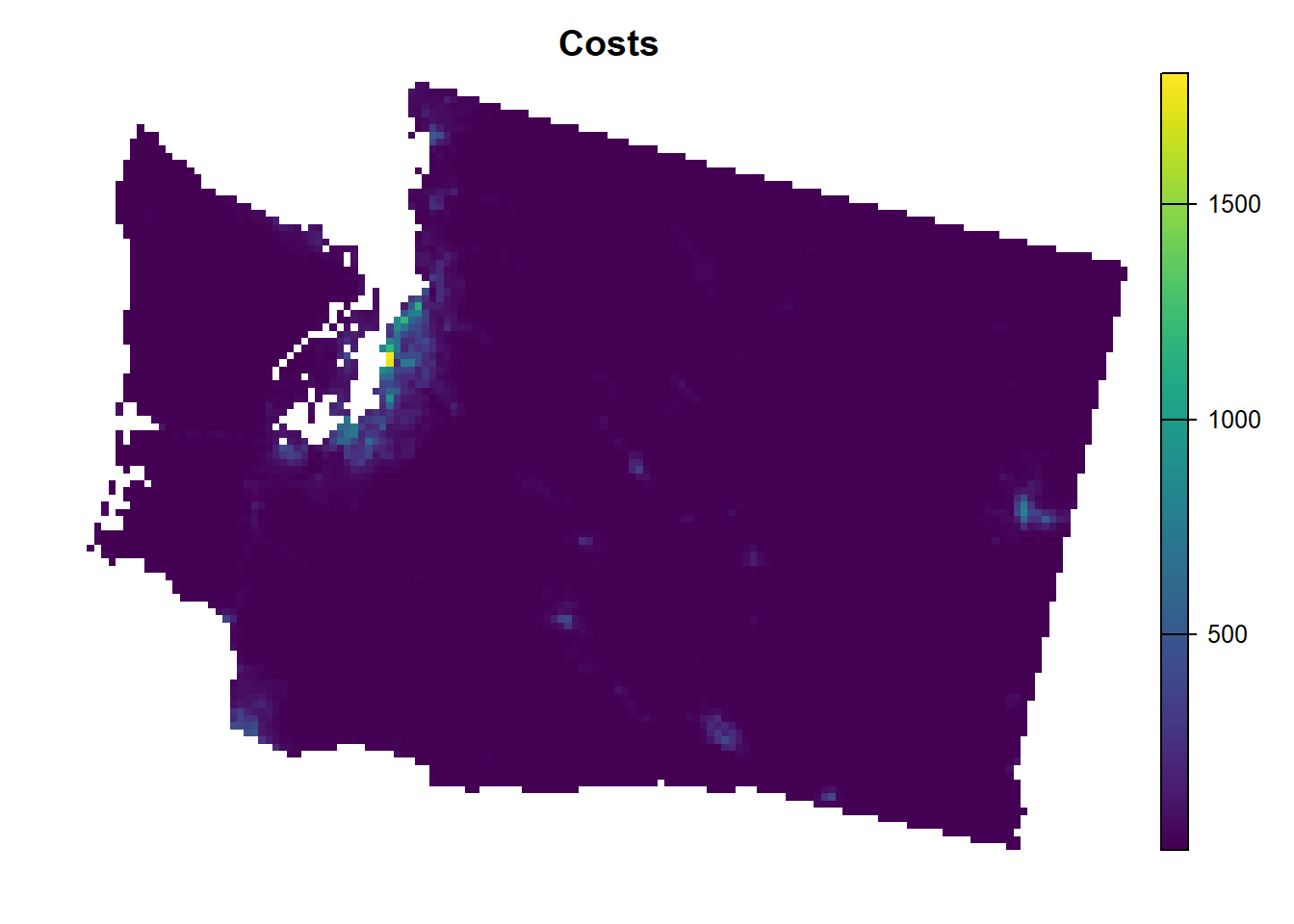
Note that this PU raster has costs built in (in this case land acquisition costs). There are a total of 10,757 PUs in this raster, which is at the 4 x 4 kilometer resolution.
7.2.2 Step 2: Species data (target features)
The next step is to identify the conservation features that are being targeted. In this case, it is the spatial distribution of birds at the same resolution as the PU raster above.
## class       : SpatRaster
## dimensions  : 109, 147, 396  (nrow, ncol, nlyr)
## resolution  : 4000, 4000  (x, y)
## extent      : -1816382, -1228382, 247483.5, 683483.5  (xmin, xmax, ymin, ymax)
## coord. ref. : +proj=laea +lat_0=45 +lon_0=-100 +x_0=0 +y_0=0 +ellps=sphere +units=m +no_defs
## source      : wa_features.tif
## names       : Recur~ding), Botau~ding), Botau~ding), Corvu~ding), Corvu~ding), Cincl~full), ...
## min values  :       0.000,       0.000,       0.000,       0.000,       0.000,        0.00, ...
## max values  :       0.514,       0.812,       3.129,       0.115,       0.296,        0.06, ...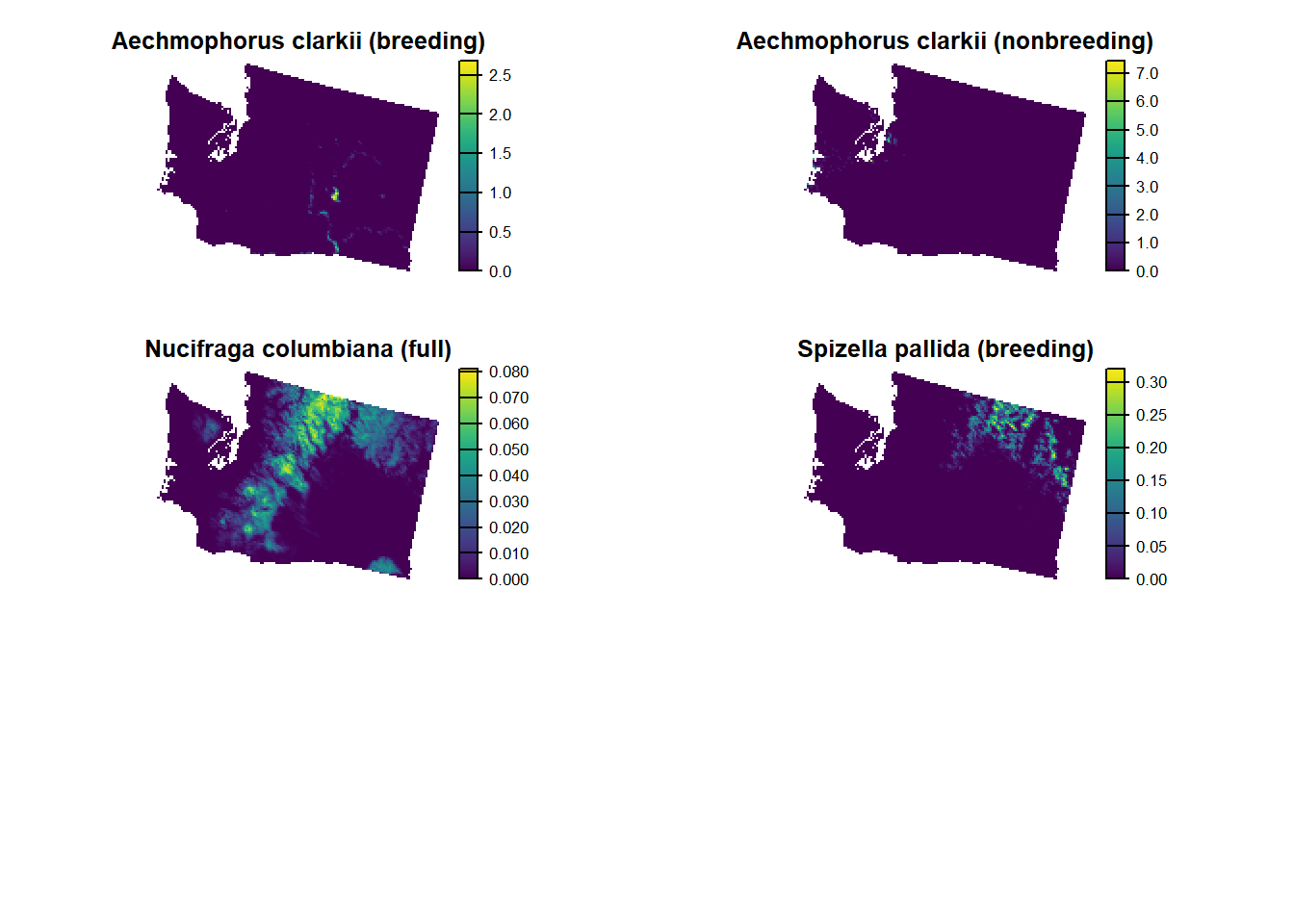
7.2.3 Step 3: Set targets
Your targets is one half of the optimization problem and the objectives/costs are the other, with everything else you can visualize as a constraint or a modifier. There are multiple ways to set targets in the package such as:
add_relative_targets() - Set proportional target (between 0 and 1) of the maximum level of representation of features (bird ranges here) in the study area, including areas that are locked out. You may set this as a single value (e.g., 20%) where you are targeting covering with the PUs 20% of each bird species range (breeding and non-breeding).
7.2.4 Step 4: Set objective (budget)
In this case our objective will be a specific budget (3917.63). For a different problem, this could be hours of management or sampling. Alternatively, there are other objective functions within the package, for example maximizing some utility that could be used for an objective like harvest.
7.2.5 Step 5: Specify the problem
While there are additional components we can add, we now have all of the pieces to set up a basic problem to find an optimal solution for. We must specify the pieces of the problem from all of the components we have brought in:
# Specify your problem
p1 <-problem(wa_pu, features = wa_bird) %>% # Our problem is for WA planning units looking at birds
  add_min_shortfall_objective(budget) %>% # Minimize shortfall (going below our target) based on budget
  add_relative_targets(target) %>% # Add our 20% target from above
  add_binary_decisions() %>% # Specify our decision is binary (buy or not buy a PU)
  add_default_solver(gap = 0.25, verbose = FALSE) # While we can solve this exactly, I am adding a gap of 25% here otherwise this takes a long time to run just for demonstration.

print(p1)
## A conservation problem (<ConservationProblem>)
## ├•data
## │├•features: "Recurvirostra americana (breeding)", … (396 total)
## │└•planning units:
## │ ├•data: <SpatRaster> (10757 total)
## │ ├•costs: continuous values (between 0.298664689064026 and 1804.18383789062)
## │ ├•extent: -1816381.61816, 247483.52106, -1228381.61816, 683483.52106 (xmin, ymin, xmax, ymax)
## │ └•CRS: +proj=laea +lat_0=45 +lon_0=-100 +x_0=0 +y_0=0 +ellps=sphere +units=m +no_defs (projected)
## ├•formulation
## │├•objective: minimum shortfall objective (`budget` = 3917.63)
## │├•penalties: none specified
## │├•targets: relative targets (between 0.2 and 0.2)
## │├•constraints: none specified
## │└•decisions: binary decision
## └•optimization
## ├•portfolio: default portfolio
## └•solver: highs solver (`gap` = 0.25, `time_limit` = 2147483647, …)
## # ℹ Use `summary(...)` to see complete formulation.We can see a nice breakdown of the components of our problem and confirm the pieces of our problem (as well as see other things we can add to our formulation).
7.2.6 Step 6: Solve!
This will by default use the “best” solver installed on your system (we installed HiGHS - high performance software for linear optimization) above so it will use this unless you have others installed.
## solution_1
##      56.74
Plot the solution:
7.2.7 Optional 1: Add Constraints
Alternatively, we can add constraints to our problem since in conservation we often aren’t considering all PUs to be possible (we may want to lock these out) and some areas may already be conserved (“locked in”). For this case study, they used the USGS Protected Areas Database of the United States (PAD-US) dataset as areas already conserved:
Lock in PUs:
# Import locked in data
wa_locked_in <- get_wa_locked_in()

# Plot data
plot(wa_locked_in, main = "Existing protected areas", axes = FALSE)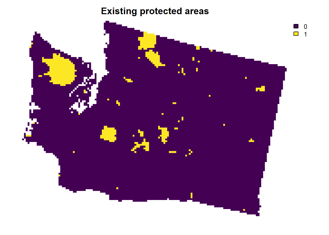
For example, you can see the large protected area of Olympic National Park in the northwest on the Olympic Peninsula.
In this case study, they “locked out” urban areas and tribal lands as places that would not be in consideration for the SCP.
Lock out PUS:
# Import locked in data
wa_locked_out <- get_wa_locked_out()

# Plot data
plot(wa_locked_out, main = "Areas not available", axes = FALSE)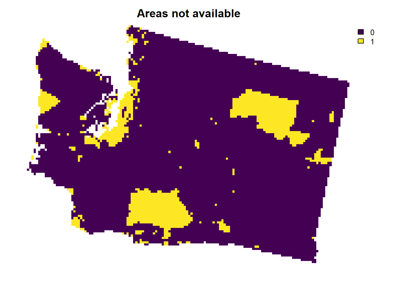
7.2.8 Optional 2: Add Penalties
The most common additional penalty is a boundary penalty, but there are many other penalties you can add. E.g., you can use add_linear_penalties() with a raster to add a linear penalty for selecting a PU based on the values of that raster (e.g., for this case it could be a measure of human disturbance to PU habitats).
Adding a boundary length modifier penalty will penalize PU solutions with more edge and less contiguous patches:
7.2.9 Putting it all together
We can then respecify our model with our constraints and penalties:
# Specify your problem
p2 <-problem(wa_pu, features = wa_bird) %>% # Our problem is for WA planning units looking at birds
  add_min_shortfall_objective(budget) %>% # Minimize shortfall (going below our target) based on budget
  add_relative_targets(target) %>% # Add our 20% target from above
  add_binary_decisions() %>% # Specify our decision is binary (buy or not buy a PU)
  add_default_solver(gap = 0.25, verbose = FALSE) %>% # While we can solve this exactly, I am adding a gap of 25% here otherwise this takes a long time to run just for demonstration.
  add_locked_in_constraints(wa_locked_in) %>% # Add locked in areas
  add_locked_out_constraints(wa_locked_out) %>% # Add locked out areas
  add_boundary_penalties(penalty = blm_penalty) # Add boundary penalty
print(p2)
## A conservation problem (<ConservationProblem>)
## ├•data
## │├•features: "Recurvirostra americana (breeding)", … (396 total)
## │└•planning units:
## │ ├•data: <SpatRaster> (10757 total)
## │ ├•costs: continuous values (between 0.298664689064026 and 1804.18383789062)
## │ ├•extent: -1816381.61816, 247483.52106, -1228381.61816, 683483.52106 (xmin, ymin, xmax, ymax)
## │ └•CRS: +proj=laea +lat_0=45 +lon_0=-100 +x_0=0 +y_0=0 +ellps=sphere +units=m +no_defs (projected)
## ├•formulation
## │├•objective: minimum shortfall objective (`budget` = 3917.63)
## │├•penalties:
## ││└•1: boundary penalties (`penalty` = 0.005, `edge_factor` = 0.5, …)
## │├•targets: relative targets (between 0.2 and 0.2)
## │├•constraints:
## ││├•1: locked in constraints (555 planning units)
## ││└•2: locked out constraints (1399 planning units)
## │└•decisions: binary decision
## └•optimization
## ├•portfolio: default portfolio
## └•solver: highs solver (`gap` = 0.25, `time_limit` = 2147483647, …)
## # ℹ Use `summary(...)` to see complete formulation.Solve again
# Solve the problem
s2 <- solve(p2)
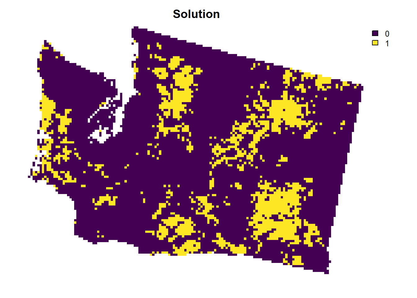
# Plot the solution w/ constraints and penalties
plot(s2, main = "Solution", axes = FALSE)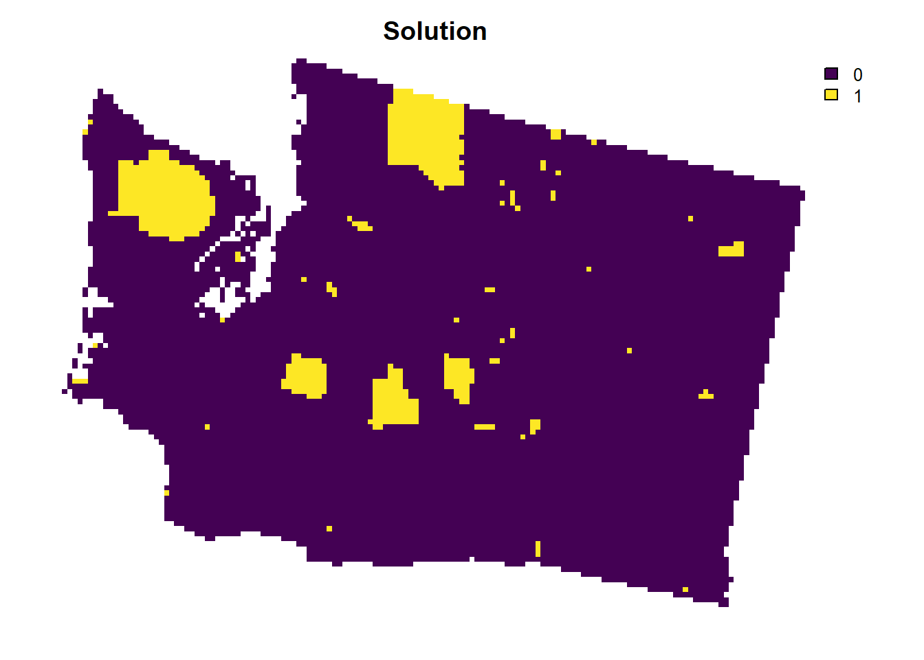
7.2.10 Additional metrics
Number of selected PUs:
## # A tibble: 1 × 2
##   summary     n
##   <chr>   <dbl>
## 1 overall   748
Total cost (in this case we optimized for cost):
## # A tibble: 1 × 2
##   summary  cost
##   <chr>   <dbl>
## 1 overall 3918.
Probably the most important output other than the PU selection is to inspect how well you fit the targets. You can see in this case, even though we got an optimization for our problem, it was impossible to meet all of our targets given our budget constraints.
## # A tibble: 6 × 9
##   feature    met   total_amount absolute_target absolute_held absolute_shortfall
##   <chr>      <lgl>        <dbl>           <dbl>         <dbl>              <dbl>
## 1 Recurviro… FALSE        100.             20.0         1.65               18.4
## 2 Botaurus … FALSE         99.9            20.0         1.01               19.0
## 3 Botaurus … FALSE        100.             20.0         3.75               16.3
## 4 Corvus br… FALSE         99.9            20.0         1.41               18.6
## 5 Corvus br… FALSE         99.9            20.0         0.623              19.4
## 6 Cinclus m… FALSE        100.             20.0        13.2                 6.78
## # ℹ 3 more variables: relative_target <dbl>, relative_held <dbl>,
## # relative_shortfall <dbl>##
## FALSE TRUE
## 393 3