Continuous variable: A numeric variable that is at least nominally continuous. (Qualitative response variables and count response variables require other regression models. See ?sec-chap06.)
Independence: The observations of the variables for one case are independent of the observations for all other cases. (If cases are dependent, linear mixed-effects models may be more appropriate. See ?sec-chap07.)
Linearity: The dependence of the response on the predictors is through the conditional expected value or mean function. (The {car} package contains many functions that can help you decide whether the assumption of linearity is reasonable in any given problem. See ?sec-chap08.)
Constant conditicional variance: The conditional variance of the response given the regressors (or, equivalently, the predictors) is constant. (See ?sec-chap05-1 — ?sec-chap05-3 and ?sec-chap08-5 for diagnostics tools.)
Changing assumptions changes the model. For example, it is common to add a normality assumption, producing the normal linear model. Another common extension to the linear model is to modify the constant variance assumption producing the weighted linear model.
4.2 Linear least-square regression
4.2.1 Simple linear regression
The Davis data set in the {carData} package contains the measured and selfreported heights and weights of 200 men and women engaged in regular exercise. A few of the data values are missing, and consequently there are only 183 complete cases for the variables that are used in the analysis reported below.
The variables weight (measured weight) and repwt (reported weight) are in kilograms, and height (measured height) and repht (reported height) are in centimeters. We focus here on the regression of weight on repwt.
R Code 4.2 : Simple linear regression of Davis data
Listing / Output 4.2: Simple linear regression model of the Davis data
Code
glue::glue("Standard call of the lm function")(davis_lm0<-lm(weight~repwt, data =Davis))save_data_file("chap04", davis_lm0, "davis_lm0.rds")glue::glue("")glue::glue("################################################################")glue::glue("Suppressing the intercept to force the regression through the origin")lm(weight~-1+repwt, data =Davis)
#> Standard call of the lm function
#>
#> Call:
#> lm(formula = weight ~ repwt, data = Davis)
#>
#> Coefficients:
#> (Intercept)        repwt
#>      5.3363       0.9278
#>
#>
#> ################################################################
#> Suppressing the intercept to force the regression through the origin
#>
#> Call:
#> lm(formula = weight ~ -1 + repwt, data = Davis)
#>
#> Coefficients:
#> repwt
#> 1.006
A model formula consists of three parts:
The left-hand side of the model formula specifies the response variable; it is usually a variable name (weight, in the example) but may be an expression that evaluates to the response (e.g., sqrt(weight), log(income), or income/hours.worked).
The tilde is a separator.
The right-hand side is the most complex part of the formula. It is a special expression, including the names of the predictors, that R evaluates to produce the regressors for the model. **The arithmetic operators, +, -, *, /, and ^, have special meaning on the right-hand side of a model formula, but they retain their ordinary meaning on the left-hand side of the formula.** R will use any unadorned numeric predictor on the right-hand side of the model formula as a regressor, as is desired here for simple regression. The intercept \(\beta_{0}\) is included in the model without being specified directly.
We can suppress the intercept to force the regression through the origin using weight ~ -1 + repwt or weight ~ repwt - 1. More generally, a minus sign removes a term, here the intercept, from the predictor. Using \(0\) (zero) also suppresses the intercept. That \(0\) is an equivalent of \(-1\) can be seen in the repetition of the formula which uses \(0\) although I have used in the formula \(-1\).
The stats::lm() function returns a linear-model object, which was assigned to the R variable davis_lm0. Printing this object just results in a relatively sparse output: Printing a linear-model object simply shows the command that produced the model along with the estimated regression coefficients.
Caution 4.1: Difference in coefficient without intercept
There is a small difference in the coefficient with and without intercept. Where does this come from and what does it mean?
Is this the result “to force the regression through the origin”?
R Code 4.3 : Summary of the linear model davis_lm0
Listing / Output 4.3: Using stats::summary() for the davis_lm0 object
#> Call: lm(formula = weight ~ repwt, data = Davis)
#>
#> Coefficients:
#>             Estimate Std. Error t value Pr(>|t|)
#> (Intercept)   5.3363     3.0369   1.757   0.0806
#> repwt         0.9278     0.0453  20.484   <2e-16
#>
#> Residual standard deviation: 8.419 on 181 degrees of freedom
#>   (17 observations deleted due to missingness)
#> Multiple R-squared: 0.6986
#> F-statistic: 419.6 on 1 and 181 DF,  p-value: < 2.2e-16
#>     AIC     BIC
#> 1303.06 1312.69
As a subset of the stats:summary() printout it does not report the residual distribution but adds with AIC and BIC two diagnostics figures for compare and choose between different models.
Call: A brief header is printed first, repeating the command that created the regression model.
Coefficients: The part of the output marked Coefficients provides basic information about the estimated regression coefficients.
The row names (=first column) lists the names of the regressors fit by lm().
Intercept: The intercept, if present, is named (Intercept).
Estimate: The column labeled Estimate provides the least-squares estimates of the regression coefficients.
Std. Error: The column marked Std. Error displays the standard errors of the estimated coefficients. The default standard errors are computed as \(\sigma\) times a function of the regressors, as presented in any regression text, but the car::S() function also allows you to use other methods for computing standard errors.
t-value: The column marked t value is the ratio of each estimate to its standard error and is a Wald test statistic for the null hypothesis that the corresponding population regression coefficient is equal to zero. If assumptions hold and the errors are normally distributed or the sample size is large enough, then these t-statistics computed with the default standard error estimates are distributed under the null hypothesis as t random variables with degrees of freedom (df ) equal to the residual degrees of freedom under the model.
Pr (>|t|): The column marked Pr (>|t|) is the two-sided p-value for the null hypothesis assuming that \(\beta_{0} = 0\) versus \(\beta_{0} \neq 0\) the t-distribution is appropriate. (Example: The hypothesis \(\beta_{0} = 0\) versus \(\beta_{0} != 0\), with the value of \(\beta_{1}\) unspecified, has a p-value of about .08, providing weak evidence against the null hypothesis that \(\beta_{0} = 0\), if the assumptions of the model hold.)
Below the coefficient table is additional summary information, including the residual standard deviation. (Example: This typical error in prediction is so large that, if correct, it is unlikely that the predictions of actual weight from reported weight would be of any practical value.)
The residual df are n − 2 for simple regression, here 183 − 2 = 181, and we’re alerted to the fact that 17 cases are removed because of missing data.
The Multiple R-squared, \(R^2 \approx 0.70\), is the square of the correlation between the response and the fitted values and is interpretable as the proportion of variation of the response variable around its mean accounted for by the regression.
F-statistic: The reported F-statistic provides a likelihood-ratio test of the general null hypothesis that all the population regression coefficients, except for the intercept, are equal to zero, versus the alternative that at least one of the \(\beta_{j}\) is nonzero. If the errors are normal or n is large enough, then this test statistic has an F-distribution with the degrees of freedom shown. Because simple regression has only one parameter beyond the intercept, the F-test is equivalent to the t-test that \(\beta_{1} = 0\), with \(t_{2} = F\). (In other models, such as GLMs or normal nonlinear models, Wald tests and the generalization of the likelihood-ratio F-test may test the same hypotheses, but they need not provide the same inferences.)
The AIC and BIC values at the bottom of the output are, respectively, the Akaike Information Criterion and the Bayesian Information Criterion, statistics that are sometimes used for model selection.
Note 4.1
With the exception of the AIC and BIC values I cannot see any advantage in the default version of car::S() against base::summary(). I am curious what it means that car::S() “adds more functionality”.
One obviously is, that car::S() allows different methods to compute standard errors.
R Code 4.5 : Short summary of the lm object with car::brief()
Listing / Output 4.5: Brief summary of the lm object with car::brief()
car::brief() for a lm object prints only the first two columns of the coefficients: Estimate and Std. Error.
R Code 4.6 : Confidence intervals for the estimates of davis_lm0
Listing / Output 4.6: Confidence intervals for the estimates of davis_lm0 with stats::confint()
Code
glue::glue("Confidence intervals with `stats::confint()`")stats::confint(davis_lm0)glue::glue(" ")glue::glue("#############################################")glue::glue("Cofidence intervals with `car::Confint()`")car::Confint(davis_lm0)
The separate confidence intervals do not address the hypothesis that simultaneously\(\beta_{0} = 0\) and \(\beta_{1} = 1\) versus the alternative that either or both of the intercept and slope differ from these values.
We shoud have started with visualization of the data set! Always start with Exploratory Data Analysis (EDA)!
Example 4.2 : Exploratory Data Analysis of Davis data set
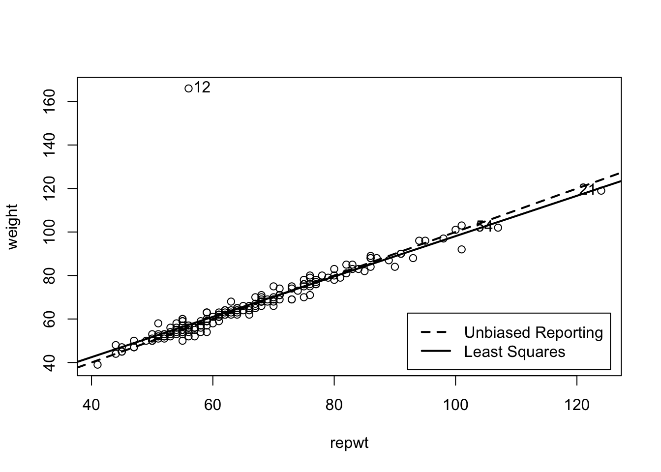
Listing / Output 4.7: Scatterplot of measured weight (weight) by reported weight (repwt) for Davis’s data. The solid line is the least-squares linear regression line, and the broken line is the line of unbiased reporting y = x.
The graphics::plot() function draws the basic scatterplot, to which we use graphics::abline() to add the line of unbiased reporting (y = x, with intercept zero and slope 1, the broken line) and the least-squares line (the solid line).
The graphics::legend() command adds a legend at the lower right of the plot, inset from the corner by 2% of the plot’s size.
The car::showLabels() function identifies the two points with the largest Mahalanobis distances from the center of the data.
The resulting graph reveals an extreme outlier, Case 12. Case 21 has also unusually large values of both measured and reported weight but is in line with the rest of the data.
It seems bizarre that an individual who weighs more than 160 kg would report her weight as less than 60 kg, but there is a simple explanation: On data entry, Subject 12’s height in centimeters and weight in kilograms were inadvertently exchanged.
R Code 4.8 : Update linar model after deleting data point 12
Listing / Output 4.8: Linear model of updated Davis data (davis_lm1)
Code
glue::glue("#####################################################")glue::glue("Updated linear model `davis_lm1`")glue::glue("#####################################################")(davis_lm1<-update(davis_lm0, subset =-12))save_data_file("chap04", davis_lm1, "davis_lm1.rds")glue::glue("#####################################################")glue::glue("Display summary with `car::S()`")glue::glue("#####################################################")glue::glue(" ")car::S(davis_lm1)
#> #####################################################
#> Updated linear model `davis_lm1`
#> #####################################################
#>
#> Call:
#> lm(formula = weight ~ repwt, data = Davis, subset = -12)
#>
#> Coefficients:
#> (Intercept)        repwt
#>      2.7338       0.9584
#>
#> #####################################################
#> Display summary with `car::S()`
#> #####################################################
#>
#> Call: lm(formula = weight ~ repwt, data = Davis, subset = -12)
#>
#> Coefficients:
#>             Estimate Std. Error t value Pr(>|t|)
#> (Intercept)  2.73380    0.81479   3.355 0.000967
#> repwt        0.95837    0.01214  78.926  < 2e-16
#>
#> Residual standard deviation: 2.254 on 180 degrees of freedom
#>   (17 observations deleted due to missingness)
#> Multiple R-squared: 0.9719
#> F-statistic:  6229 on 1 and 180 DF,  p-value: < 2.2e-16
#>    AIC    BIC
#> 816.27 825.88
R Code 4.9 : Compare coefficients and confidence intervals
Listing / Output 4.9: Using car::compareCoefs() to compare the estimated coefficients and their standard errors from the two fitted regressions, with and without Case 12, and car::Confint() to recompute the confidence intervals for the coefficients
Code
glue::glue("############################################################")glue::glue("Compare estimated coefficients of both models")glue::glue("############################################################")glue::glue(" ")car::compareCoefs(davis_lm0, davis_lm1)glue::glue(" ")glue::glue("############################################################")glue::glue("Recomputing the confidence intervals for the coefficients")glue::glue("############################################################")glue::glue(" ")car::Confint(davis_lm1)
#> ############################################################
#> Compare estimated coefficients of both models
#> ############################################################
#>
#> Calls:
#> 1: lm(formula = weight ~ repwt, data = Davis)
#> 2: lm(formula = weight ~ repwt, data = Davis, subset = -12)
#>
#>             Model 1 Model 2
#> (Intercept)   5.336   2.734
#> SE            3.037   0.815
#>
#> repwt        0.9278  0.9584
#> SE           0.0453  0.0121
#>
#>
#> ############################################################
#> Recomputing the confidence intervals for the coefficients
#> ############################################################
#>
#>              Estimate     2.5 %    97.5 %
#> (Intercept) 2.7338020 1.1260247 4.3415792
#> repwt       0.9583743 0.9344139 0.9823347
Both the intercept and the slope change, but not dramatically, when the outlier is removed. Case 12 is at a relatively low-leverage point, because its value for repwt is near the center of the distribution of the regressor.
In contrast, there is a major change in the residual standard deviation, reduced from an unacceptable 8.4 kg to a possibly acceptable 2.2 kg.
As a consequence, the coefficient standard errors are also much smaller when the outlier is removed, and the value of \(R^2\) is greatly increased. Because the coefficient standard errors are now smaller, even though the estimated intercept \(b_{0}\) is still close to zero and the estimated slope \(b_{1}\) is close to 1, \(b_{0} = 0\) and \(b_{1} = 1\) are both outside of the recomputed 95% confidence intervals for the coefficients1
In the following experiment I am trying to reproduce book’s Figure 4.1. I have to solve two challenges:
Calculating the Mahalanobis distances and returning the farest distances.
Applying these values and printing out the row names (ID numbers in this case) near the coordinates of the points the belong to.
Experiment 4.1 : Interactive plot and labelled Mahalanobis distances
R Code 4.10 : Simple linear regression of interactive Davis data produced with {ggiraph}
Listing / Output 4.10: Interactive linear model of weight regresssed on repwt with Davis data set. Interactivity created with {ggiraph}.
Code
Davis<-carData::Davisgg_davis<-Davis|>tidyr::drop_na(repwt)|>tibble::rowid_to_column(var ="ID")|>ggplot2::ggplot(ggplot2::aes( x =repwt, y =weight))+ggiraph::geom_point_interactive(ggplot2::aes( x =repwt, y =weight, tooltip =ID, data_id =ID), shape =1, size =2)+ggplot2::geom_smooth(ggplot2::aes( linetype ="solid"), formula =y~x, method =lm, se =FALSE, color ="black")+ggplot2::geom_smooth(ggplot2::aes( linetype ="dashed",), formula =y~x, method =loess, se =FALSE, color ="black")+ggplot2::scale_linetype_discrete( name ="", label =c("Least Squares","Unbiased Reporting "))+ggplot2::guides( linetype =ggplot2::guide_legend(position ="inside"))+ggplot2::theme( legend.title =ggplot2::element_blank(), legend.position.inside =c(.8, .15), legend.box.background =ggplot2::element_rect( color ="black", linewidth =1))ggiraph::girafe(ggobj =gg_davis)
This was my first try to replicate the book’s Figure 4.1. There are two important qualification to make:
1. Producing an interactive graphics with {ggiraph}
Instead of printing out the two points with the largest Mahalanobis distance I have applied functions from the {ggiraph} package to produce an interactive plot. When you hover the cursor over data points you will get a tooltip with the row number of the point under your cursor. After you learned that the outlier with weight over 160kg is from row 12 you can delete this data point in the next step.
I used {ggiraph} for two reasons:
(a) {ggigraph} is easy to use
{ggiraph} (see Package Profile A.7) uses the {ggplot2} structure and names of commands. There are only three changes for making a {ggplot2} graph interactive:
Provide at least one of the aesthetics tooltip, data_id and onclick to create interactive elements.
Call function ggiraph::girafe() with the ggplot object so that the graphic is translated as a web interactive graphics.
It wasn’t therefore necessary to invest much time for learning a new package as it would have been the case for learning {plotly}, another package for creating interactive web graphics (see Package Profile A.16).
(b) At first I didn’t know how to calculate Mahalanobis distances
I knew I could use the {ggrepel} package (see Package Profile A.9) to label the points but I didn’t know how to calculate the two points with the largest Mahalanobis distance. Although I knew that there is in base R the stats::mahalanobis() function, but at first I didn’t succeed to provide the necessary parameter for the arguments. Some days later I found the solution with Listing / Output 4.11.
2. New detailed specification for the {ggplot2} legend
R Code 4.11 : Simple linear regression of weight on repwt with labelled points of the biggest Mahalanobis distances using {ggrepel}
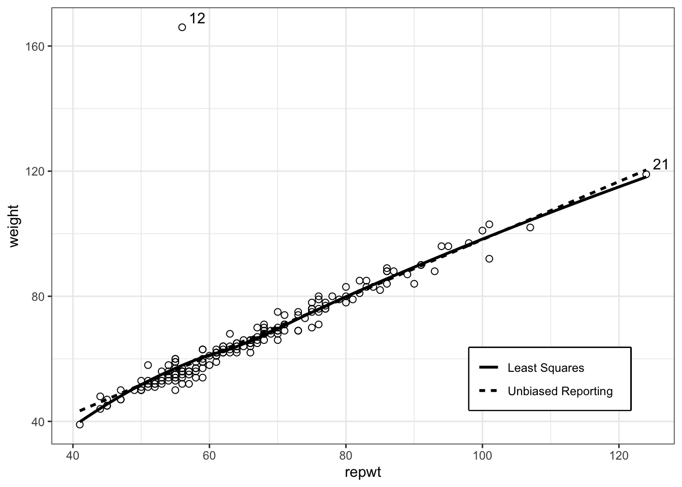
Listing / Output 4.11: Replication of book’s Figure 4.1 with {ggplot2} and {ggrepel}
Code
set.seed(420)df_temp<-carData::Davis|>dplyr::select(weight, repwt)|>tidyr::drop_na()df<-df_temp|>dplyr::mutate(mahal ={stats::mahalanobis(df_temp,base::colMeans(df_temp),stats::cov(df_temp))})|>dplyr::mutate(p =pchisq( q =mahal, df =1, lower.tail =FALSE))|>tibble::rownames_to_column(var ="ID")|>dplyr::mutate(ID =dplyr::case_when(p<.001~ID,p>=.001~""))df|>ggplot2::ggplot(ggplot2::aes( x =repwt, y =weight))+ggplot2::geom_point( shape =1, size =2)+ggrepel::geom_text_repel(ggplot2::aes(label =ID))+ggplot2::stat_smooth(ggplot2::aes(linetype ="solid"), formula =y~x, method =lm, se =FALSE, color ="black")+ggplot2::geom_smooth(ggplot2::aes( linetype ="dashed"), formula =y~x, method =loess, se =FALSE, color ="black")+ggplot2::scale_linetype_discrete( name ="", label =c("Least Squares","Unbiased Reporting "))+ggplot2::guides( linetype =ggplot2::guide_legend(position ="inside"))+ggplot2::theme( legend.title =ggplot2::element_blank(), legend.position.inside =c(.8, .15), legend.box.background =ggplot2::element_rect( color ="black", linewidth =1))
This is my best attempt to replicate book’s Figure 4.1. Instead of using functions of tthe he {car} package I used packages from the {tidyverse} approach: {gplot2} and {ggrepel} (see Package Profile A.9).
Resource 4.1 : Mahalanobis Distance
I didn’t know that stats::mahalanobis() requires as parameters the dataframe with the regression variables. Two almost identical blog articles showed me how to apply the base R function:
Finnstats: How to Calculate Mahalanobis Distance in R (I believe that this article was the original of the two.)
Statology: How to Calculate Mahalanobis Distance in R
The Mahalanobis distance is a distance measure of multivariate distributions and was developed 1936 by Prasanta Chandra Mahalanobis. In contrast to the Euclidean distance which works fine as long as the dimensions are equally weighted and are independent of each other, the Mahalanobis distance takes into account different axis variances and correlation.
Very instructive for me was the (German) article Mahalanobis-Distanz. It features an experiment where a graphic shows that the distances from different points on a circle with the center in the data cloud are not equal because of different standard deviations on different axes. Mahalanobis distance takes into account the different standard deviations along the axes of the n-dimensional space as well as the correlation (variances and covariances) between the axes.
During the work with {ggrepel} I encountered another difficulty receiving several {ggplot2} warnings. I could finally solve this problem after asking about help on StackOverflow.
4.3 Multiple linear regression
Multiple regression extends simple regression to more than one predictor.
The estimated regression coefficient replaces the Greek letter with the corresponding Roman letter, as in \(b_{1}\) for \(\beta_{1}\).↩︎
Source Code
# Fitting linear models {#sec-chap04}```{r}#| label: setup#| results: hold#| include: falsebase::source(file ="R/helper.R")ggplot2::theme_set(ggplot2::theme_bw())options(show.signif.stars =FALSE)```## Table of content for chapter 04 {.unnumbered}::::: {#obj-chap04}:::: {.my-objectives}::: {.my-objectives-header}Chapter section list:::::: {.my-objectives-container}- The linear model (@sec-chap04-1)- Linear least-square regression (@sec-chap04-2) - Simple linear regression (@sec-chap04-2-1) - Multiple linear regression (@sec-chap04-2-2)::::::::::::## The linear model {#sec-chap04-1}:::{.my-bulletbox}:::: {.my-bulletbox-header}::::: {.my-bulletbox-icon}::::::::::: {#bul-chap04-lm-assumptions}::::::: Assumption of the linear model:::::::: {.my-bulletbox-body}The assumptions of the linear models are:- **Continuous variable**: A numeric variable that is at least nominally continuous. (Qualitative response variables and count response variables require other regression models. See @sec-chap06.)- **Independence**: The observations of the variables for one case are independent of the observations for all other cases. (If cases are dependent, linear mixed-effects models may be more appropriate. See @sec-chap07.)- **Linearity**: The dependence of the response on the predictors is through the conditional expected value or *mean function*. (The {**car**} package contains many functions that can help you decide whether the assumption of linearity is reasonable in any given problem. See @sec-chap08.)- **Constant conditicional variance**: The conditional variance of the response given the regressors (or, equivalently, the predictors) is constant. (See @sec-chap05-1 --- @sec-chap05-3 and @sec-chap08-5 for diagnostics tools.)***Changing assumptions changes the model. For example, it is common to add a normality assumption, producing the *normal linear model*. Another common extension to the linear model is to modify the constant variance assumption producing the *weighted linear model*. :::::::## Linear least-square regression {#sec-chap04-2}### Simple linear regression {#sec-chap04-2-1}The Davis data set in the {**carData**} package contains the measured and selfreported heights and weights of 200 men and women engaged in regular exercise. A few of the data values are missing, and consequently there are only 183 complete cases for the variables that are used in the analysis reported below.The variables `weight` (measured weight) and `repwt` (reported weight) are in kilograms, and `height` (measured height) and `repht` (reported height) are in centimeters. We focus here on the regression of `weight` on `repwt.`:::::{.my-example}:::{.my-example-header}:::::: {#exm-chap04-lm-davis}: Simple linear regression :::::::::::::{.my-example-container}::: {.panel-tabset}###### Davis:::::{.my-r-code}:::{.my-r-code-header}:::::: {#cnj-chap04-skim-Davis-data}: A quick look at the Davis data:::::::::::::{.my-r-code-container}::: {#lst-chap04-skim-Davis-data}```{r}#| label: skim-Davis-dataDavis <- carData::Davisskimr::skim(Davis)```Skim the Davis data set:::***Instead of using the `base::summary()` function I have applied the `skim()` function from the {**skimr**} package. See @pak-skimr.:::::::::###### davis_lm0:::::{.my-r-code}:::{.my-r-code-header}:::::: {#cnj-chap04-print-davis-lm0}: Simple linear regression of Davis data:::::::::::::{.my-r-code-container}::: {#lst-chap04-print-davis-lm0}```{r}#| label: print-davis-lm0#| results: holdglue::glue("Standard call of the lm function")(davis_lm0 <-lm(weight ~ repwt, data = Davis))save_data_file("chap04", davis_lm0, "davis_lm0.rds")glue::glue("")glue::glue("################################################################")glue::glue("Suppressing the intercept to force the regression through the origin")lm(weight ~-1+ repwt, data = Davis)```Simple linear regression model of the Davis data:::***A model formula consists of three parts: - 1. **The left-hand side** of the model formula specifies the response variable; it is usually a variable name (`weight`, in the example) but may be an expression that evaluates to the response (e.g., `sqrt(weight)`, `log(income)`, or `income/hours.worked`). - 2. **The tilde** is a separator. - 3. **The right-hand side** is the most complex part of the formula. It is a special expression, including the names of the predictors, that R evaluates to produce the regressors for the model. **The arithmetic operators, +, -, *, /, and ^, have special meaning on the right-hand side of a model formula, but they retain their ordinary meaning on the left-hand side of the formula.** R will use any unadorned numeric predictor on the right-hand side of the model formula as a regressor, as is desired here for simple regression. The intercept $\beta_{0}$ is included in the model without being specified directly.We can suppress the intercept to force the regression through the origin using `weight ~ -1 + repwt` or `weight ~ repwt - 1`. More generally, a minus sign removes a term, here the intercept, from the predictor. Using $0$ (zero) also suppresses the intercept. That $0$ is an equivalent of $-1$ can be seen in the repetition of the formula which uses $0$ although I have used in the formula $-1$.The `stats::lm()` function returns a linear-model object, which was assigned to the R variable `davis_lm0`. Printing this object just results in a relatively sparse output: Printing a linear-model object simply shows the command that produced the model along with the estimated regression coefficients.::: {.callout-caution style="color: darkgoldenrod;" #cau-chap04-without-intercept}##### Difference in coefficient without interceptThere is a small difference in the coefficient with and without intercept. Where does this come from and what does it mean?Is this the result "to force the regression through the origin"?::::::::::::###### stats::summary():::::{.my-r-code}:::{.my-r-code-header}:::::: {#cnj-summary-davis-lm0}: Summary of the linear model `davis_lm0`:::::::::::::{.my-r-code-container}::: {#lst-listing-ID} ```{r}#| label: summary-davis-lm0summary(davis_lm0)```Using stats::summary() for the `davis_lm0` object:::***For an explication of the different printed parts see @lst-chap04-car-S-davis-lm0.:::::::::###### car::S():::::{.my-r-code}:::{.my-r-code-header}:::::: {#cnj-chap04-car-S-davis-lm0}: Default usage of the more sophisticated summary with `car::S()`:::::::::::::{.my-r-code-container}::: {#lst-chap04-car-S-davis-lm0}```{r}#| label: S-davis-lm0car::S(davis_lm0)```Default summary output of `car::S()`:::***As a subset of the stats:summary() printout it does not report the residual distribution but adds with AIC and BIC two diagnostics figures for compare and choose between different models.- **Call**: A brief header is printed first, repeating the command that created the regression model. - **Coefficients**: The part of the output marked `Coefficients` provides basic information about the estimated regression coefficients. - The **row names** (=first column) lists the names of the regressors fit by `lm()`. - **Intercept**: The intercept, if present, is named `(Intercept)`. - **Estimate**: The column labeled `Estimate` provides the least-squares estimates of the regression coefficients. - **Std. Error**: The column marked `Std. Error` displays the standard errors of the estimated coefficients. The default standard errors are computed as $\sigma$ times a function of the regressors, as presented in any regression text, but the `car::S()` function also allows you to use other methods for computing standard errors. - **t-value**: The column marked `t value` is the ratio of each estimate to its standard error and is a `r glossary("Wald", "Wald test statistic")` for the null hypothesis that the corresponding population regression coefficient is equal to zero. If assumptions hold and the errors are normally distributed or the sample size is large enough, then these `r glossary("t-statistic", "t-statistics")` computed with the default `r glossary("standard error")` estimates are distributed under the null hypothesis as t random variables with `r glossary("degrees of freedom")` (df ) equal to the `r glossary("Residually", "residual")` degrees of freedom under the model. - **Pr (>|t|)**: The column marked `Pr (>|t|)` is the two-sided `r glossary("p-value")` for the null hypothesis assuming that $\beta_{0} = 0$ versus $\beta_{0} \neq 0$ the t-distribution is appropriate. (*Example*: The hypothesis $\beta_{0} = 0$ versus $\beta_{0} != 0$, with the value of $\beta_{1}$ unspecified, has a p-value of about .08, providing weak evidence against the null hypothesis that $\beta_{0} = 0$, if the assumptions of the model hold.) - Below the coefficient table is additional summary information, including the **residual standard deviation**. (*Example*: This typical error in prediction is so large that, if correct, it is unlikely that the predictions of actual weight from reported weight would be of any practical value.) - The **residual df** are n − 2 for simple regression, here 183 − 2 = 181, and we’re alerted to the fact that 17 cases are removed because of missing data. - The **Multiple R-squared**, $R^2 \approx 0.70$, is the square of the correlation between the response and the fitted values and is interpretable as the proportion of variation of the response variable around its mean accounted for by the regression. - **F-statistic**: The reported `r glossary("F-statistic")` provides a `r glossary("likelihood-ratio")` test of the general null hypothesis that all the population regression coefficients, except for the intercept, are equal to zero, versus the alternative that at least one of the $\beta_{j}$ is nonzero. If the errors are normal or n is large enough, then this test statistic has an F-distribution with the degrees of freedom shown. Because simple regression has only one parameter beyond the intercept, the F-test is equivalent to the t-test that $\beta_{1} = 0$, with $t_{2} = F$. (In other models, such as GLMs or normal nonlinear models, Wald tests and the generalization of the likelihood-ratio F-test may test the same hypotheses, but they need not provide the same inferences.) - The **AIC** and **BIC** values at the bottom of the output are, respectively, the Akaike Information Criterion and the Bayesian Information Criterion, statistics that are sometimes used for model selection.:::::::::::: {.callout-note style="color: blue;" #nte-chap04-S-versus-summary}With the exception of the AIC and BIC values I cannot see any advantage in the default version of `car::S()` against `base::summary()`. I am curious what it means that car::S() "adds more functionality".One obviously is, that car::S() allows different methods to compute standard errors.:::###### car::brief():::::{.my-r-code}:::{.my-r-code-header}:::::: {#cnj-chap04-car-brief-davis-lm0}: Short summary of the lm object with `car::brief()`:::::::::::::{.my-r-code-container}::: {#lst-chap04-car-brief-davis-lm0}```{r}#| label: car-brief-davis-lm0car::brief(davis_lm0)```Brief summary of the lm object with `car::brief()`:::`car::brief()` for a `lm` object prints only the first two columns of the coefficients: `Estimate` and `Std. Error`.:::::::::###### Confidence intervals:::::{.my-r-code}:::{.my-r-code-header}:::::: {#cnj-chap04-confidence-intervals-davis-lm0}: Confidence intervals for the estimates of `davis_lm0`:::::::::::::{.my-r-code-container}::: {#lst-chap04-confidence-intervals-davis-lm0}```{r}#| label: confidence-intervals-davis-lm0#| results: holdglue::glue("Confidence intervals with `stats::confint()`")stats::confint(davis_lm0)glue::glue(" ")glue::glue("#############################################")glue::glue("Cofidence intervals with `car::Confint()`")car::Confint(davis_lm0)```Confidence intervals for the estimates of `davis_lm0` with `stats::confint()`:::***Unlike `stats::confint()`, `car::Confint()` prints the coefficient estimates along with the confidence limits.:::::::::The separate confidence intervals do not address the hypothesis that *simultaneously* $\beta_{0} = 0$ and $\beta_{1} = 1$ versus the alternative that either or both of the intercept and slope differ from these values.::::::::::::We shoud have started with visualization of the data set! Always start with Exploratory Data Analysis (`r glossary("ExDA", "EDA")`)!:::::{.my-example}:::{.my-example-header}:::::: {#exm-chap04-eda}: Exploratory Data Analysis of Davis data set:::::::::::::{.my-example-container}::: {.panel-tabset}###### plot(davis_lm0):::::{.my-r-code}:::{.my-r-code-header}:::::: {#cnj-chap04-scatterplot-davis-lm0}: Scatterplot of `davis_lm0`:::::::::::::{.my-r-code-container}::: {#lst-chap04-scatterplot-davis-lm0}```{r}#| label: scatterplot-davis-lm0Davis <- carData::Davisgraphics::plot(weight ~ repwt, data = Davis)graphics::abline(0, 1, lty ="dashed", lwd =2)graphics::abline(davis_lm0, lwd =2)graphics::legend("bottomright",c("Unbiased Reporting", "Least Squares"),lty =c("dashed", "solid"),lwd =2,inset =0.02)base::with(Davis, car::showLabels(repwt, weight, n =3, method ="mahal"))```Scatterplot of measured weight (`weight`) by reported weight (`repwt`) for Davis’s data. The solid line is the least-squares linear regression line, and the broken line is the line of unbiased reporting y = x.:::***- The `graphics::plot()` function draws the basic scatterplot, to which we use `graphics::abline()` to add the line of unbiased reporting (y = x, with intercept zero and slope 1, the broken line) and the least-squares line (the solid line). - The `graphics::legend()` command adds a legend at the lower right of the plot, inset from the corner by 2% of the plot’s size. - The `car::showLabels()` function identifies the two points with the largest `r glossary("Mahalanobis")` distances from the center of the data.:::::::::The resulting graph reveals an extreme outlier, Case 12. Case 21 has also unusually large values of both measured and reported weight but is in line with the rest of the data. It seems bizarre that an individual who weighs more than 160 kg would report her weight as less than 60 kg, but there is a simple explanation: On data entry, Subject 12’s height in centimeters and weight in kilograms were inadvertently exchanged.###### update:::::{.my-r-code}:::{.my-r-code-header}:::::: {#cnj-chap04-update-davis}: Update linar model after deleting data point 12:::::::::::::{.my-r-code-container}::: {#lst-chap04-update-davis}```{r}#| label: update-davis#| results: holdglue::glue("#####################################################")glue::glue("Updated linear model `davis_lm1`")glue::glue("#####################################################")(davis_lm1 <-update(davis_lm0, subset =-12))save_data_file("chap04", davis_lm1, "davis_lm1.rds")glue::glue("#####################################################")glue::glue("Display summary with `car::S()`")glue::glue("#####################################################")glue::glue(" ")car::S(davis_lm1)```Linear model of updated Davis data (`davis_lm1`)::::::::::::###### compare models:::::{.my-r-code}:::{.my-r-code-header}:::::: {#cnj-chap04-compare-models}: Compare coefficients and confidence intervals:::::::::::::{.my-r-code-container}::: {#lst-chap04-compare-models}```{r}#| label: compare-models#| results: holdglue::glue("############################################################")glue::glue("Compare estimated coefficients of both models")glue::glue("############################################################")glue::glue(" ")car::compareCoefs(davis_lm0, davis_lm1)glue::glue(" ")glue::glue("############################################################")glue::glue("Recomputing the confidence intervals for the coefficients")glue::glue("############################################################")glue::glue(" ")car::Confint(davis_lm1)```Using `car::compareCoefs()` to compare the estimated coefficients and their standard errors from the two fitted regressions, with and without Case 12, and `car::Confint()` to recompute the confidence intervals for the coefficients::::::::::::Both the intercept and the slope change, but not dramatically, when the outlier is removed. Case 12 is at a relatively *low-leverage point*, because its value for `repwt` is near the center of the distribution of the regressor. In contrast, there is a major change in the residual standard deviation, reduced from an unacceptable 8.4 kg to a possibly acceptable 2.2 kg.As a consequence, the coefficient standard errors are also much smaller when the outlier is removed, and the value of $R^2$ is greatly increased. Because the coefficient standard errors are now smaller, even though the estimated intercept $b_{0}$ is still close to zero and the estimated slope $b_{1}$ is close to 1, $b_{0} = 0$ and $b_{1} = 1$ are both outside of the recomputed 95% confidence intervals for the coefficients[^04-fitting-lm-1][^04-fitting-lm-1]: The estimated regression coefficient replaces the Greek letter with the corresponding Roman letter, as in $b_{1}$ for $\beta_{1}$.::::::::::::In the following experiment I am trying to reproduce book’s Figure 4.1. I have to solve two challenges:1. Calculating the Mahalanobis distances and returning the farest distances.2. Applying these values and printing out the row names (ID numbers in this case) near the coordinates of the points the belong to.:::::{.my-experiment}:::{.my-experiment-header}:::::: {#def-chap04-replicating-books-figure-4-1}: Interactive plot and labelled Mahalanobis distances:::::::::::::{.my-experiment-container}::: {.panel-tabset}###### {ggiraph}:::::{.my-r-code}:::{.my-r-code-header}:::::: {#cnj-chap04-davis-ggiraph}: Simple linear regression of interactive Davis data produced with {ggiraph}:::::::::::::{.my-r-code-container}::: {#lst-chap04-davis-ggiraph} ```{r}#| label: davis-ggiraphDavis <- carData::Davisgg_davis <- Davis |> tidyr::drop_na(repwt) |> tibble::rowid_to_column(var ="ID") |> ggplot2::ggplot( ggplot2::aes(x = repwt,y = weight ) ) + ggiraph::geom_point_interactive( ggplot2::aes(x = repwt,y = weight,tooltip = ID,data_id = ID ),shape =1,size =2 ) + ggplot2::geom_smooth( ggplot2::aes(linetype ="solid" ),formula = y ~ x,method = lm,se =FALSE,color ="black" ) + ggplot2::geom_smooth( ggplot2::aes(linetype ="dashed", ),formula = y ~ x,method = loess,se =FALSE,color ="black" ) + ggplot2::scale_linetype_discrete(name ="",label =c("Least Squares","Unbiased Reporting " ) ) + ggplot2::guides(linetype = ggplot2::guide_legend(position ="inside") ) + ggplot2::theme(legend.title = ggplot2::element_blank(),legend.position.inside =c(.8, .15),legend.box.background = ggplot2::element_rect(color ="black", linewidth =1 ) )ggiraph::girafe(ggobj = gg_davis)```Interactive linear model of `weight` regresssed on `repwt` with Davis data set. Interactivity created with {**ggiraph**}.:::***This was my first try to replicate the book’s Figure 4.1. There are two important qualification to make:**1. Producing an interactive graphics with {ggiraph}** Instead of printing out the two points with the largest `r glossary("Mahalanobis")` distance I have applied functions from the {**ggiraph**} package to produce an interactive plot. When you hover the cursor over data points you will get a tooltip with the row number of the point under your cursor. After you learned that the outlier with weight over 160kg is from row 12 you can delete this data point in the next step.I used {**ggiraph**} for two reasons:**(a) {**ggigraph**} is easy to use**- {**ggiraph**} (see @pak-ggiraph) uses the {**ggplot2**} structure and names of commands. There are only three changes for making a {**ggplot2**} graph interactive: - 1. Instead of using `ggplot2::geom_point()`, use `ggiraph::geom_point_interactive()` - 2. Provide at least one of the aesthetics `tooltip`, `data_id` and `onclick` to create interactive elements. - 3. Call function `ggiraph::girafe()` with the ggplot object so that the graphic is translated as a web interactive graphics. It wasn't therefore necessary to invest much time for learning a new package as it would have been the case for learning {**plotly**}, another package for creating interactive web graphics (see @pak-plotly).**(b) At first I didn't know how to calculate `r glossary("Mahalanobis")` distances**I knew I could use the {**ggrepel**} package (see @pak-ggrepel) to label the points but I didn't know how to calculate the two points with the largest Mahalanobis distance. Although I knew that there is in base R the `stats::mahalanobis()` function, but at first I didn't succeed to provide the necessary parameter for the arguments. Some days later I found the solution with @lst-chap04-davis-ggrepel.**2. New detailed specification for the {ggplot2} legend**This is the first time, that I have moved the legend inside the graoh and framed with a box. I used the [https://tidyverse.or/blog](https://tidyverse.or/blog) article [ggplot2 3.5.0: legends](https://www.tidyverse.org/blog/2024/02/ggplot2-3-5-0-legends/) and an article from [https://r-graph-gallery.com](https://r-graph-gallery.com)[Building a nice legend with R and ggplot2](https://r-graph-gallery.com/239-custom-layout-legend-ggplot2.html). Helpful were also hints from a [StackOverflow post](https://stackoverflow.com/a/47669217/7322615). :::::::::###### {ggrepel}:::::{.my-r-code}:::{.my-r-code-header}:::::: {#cnj-chap04-davis-ggrepel}: Simple linear regression of `weight` on `repwt` with labelled points of the biggest Mahalanobis distances using {**ggrepel**}:::::::::::::{.my-r-code-container}::: {#lst-chap04-davis-ggrepel}```{r}#| label: davis-ggrepelset.seed(420)df_temp <- carData::Davis |> dplyr::select(weight, repwt) |> tidyr::drop_na() df <- df_temp |> dplyr::mutate(mahal = { stats::mahalanobis( df_temp, base::colMeans(df_temp), stats::cov(df_temp) ) } ) |> dplyr::mutate(p =pchisq(q = mahal,df =1,lower.tail =FALSE ) ) |> tibble::rownames_to_column(var ="ID") |> dplyr::mutate(ID = dplyr::case_when(p < .001~ ID, p >= .001~"") )df |> ggplot2::ggplot( ggplot2::aes(x = repwt,y = weight ) ) + ggplot2::geom_point(shape =1,size =2 ) + ggrepel::geom_text_repel( ggplot2::aes(label = ID) ) + ggplot2::stat_smooth( ggplot2::aes(linetype ="solid"),formula = y ~ x,method = lm,se =FALSE,color ="black" ) + ggplot2::geom_smooth( ggplot2::aes(linetype ="dashed" ),formula = y ~ x,method = loess,se =FALSE,color ="black" ) + ggplot2::scale_linetype_discrete(name ="",label =c("Least Squares","Unbiased Reporting " ) ) + ggplot2::guides(linetype = ggplot2::guide_legend(position ="inside") ) + ggplot2::theme(legend.title = ggplot2::element_blank(),legend.position.inside =c(.8, .15),legend.box.background = ggplot2::element_rect(color ="black",linewidth =1 ) )```Replication of book’s Figure 4.1 with {**ggplot2**} and {**ggrepel**}:::***This is my best attempt to replicate book’s Figure 4.1. Instead of using functions of tthe he {**car**} package I used packages from the {**tidyverse**} approach: {**gplot2**} and {**ggrepel**} (see @pak-ggrepel). :::::{.my-resource}:::{.my-resource-header}:::::: {#lem-chap04-mahalanobis-distance}: Mahalanobis Distance:::::::::::::{.my-resource-container}I didn't know that `stats::mahalanobis()` requires as parameters the dataframe with the regression variables. Two almost identical blog articles showed me how to apply the base R function:- **Finnstats**: How to Calculate Mahalanobis Distance in R (I believe that this article was the original of the two.)- **Statology**: How to Calculate Mahalanobis Distance in R The Mahalanobis distance is a distance measure of multivariate distributions and was developed 1936 by [Prasanta Chandra Mahalanobis.](https://en.wikipedia.org/wiki/Prasanta_Chandra_Mahalanobis) In contrast to the Euclidean distance which works fine as long as the dimensions are equally weighted and are independent of each other, the Mahalanobis distance takes into account different axis variances and correlation.Very instructive for me was the (German) article [Mahalanobis-Distanz](http://www.statistics4u.info/fundstat_germ/ee_mahalanobis_distance.html). It features an experiment where a graphic shows that the distances from different points on a circle with the center in the data cloud are not equal because of different standard deviations on different axes. Mahalanobis distance takes into account the different standard deviations along the axes of the n-dimensional space as well as the correlation (variances and covariances) between the axes.::::::::::::::::::During the work with {**ggrepel**} I encountered another difficulty receiving several {**ggplot2**} warnings. I could finally solve this problem after asking about [help on StackOverflow](https://stackoverflow.com/questions/78551672/ggplot2geom-smooth-drops-aesethetics-label-with-ggrepel/78552354?noredirect=1#comment138488632_78552354).::::::::::::## Multiple linear regression {#sec-chap04-2-2}Multiple regression extends simple regression to more than one predictor.