A novel feature of the R help system is the facility it provides to execute most examples in the help pages via the utils::example() command: \[example('log')\]
A quick way to determine the arguments of an R function is to use the args() function: \[args('log')\]
Warning 1.1
args() and help() functions may not be very helpful with generic functions.
For the full set of reserved symbols in R, see \[help('Reserved')\]
There are two types of logical operators:
vectorizes: \(\&\) and \(|\) vectorized resp.
single operand: \(\&\&\) and \(||\)
The unvectorized versions of the and (&&) and or (||) operators are primarily useful for writing R programs and are not appropriate for indexing vectors.
1.4 Fixing errors and getting help
Bullet List 1.1
: Getting help
base::traceback() provides information about the sequence of function calls leading up to an error.
utils::apropos('<searchString>') searches for currently accessible objects whose names contain a particular character string. It returns a character vector giving the names of objects in the search list matching (as a regular expression)
utils:find('<searchString>') returns where objects of a given name can be found.
?? or help.search() activates a broader search because it looks not only in the title fields but in other fields of the help pages as well.
utils::RSiteSearch() or the search engine at https://search.r-project.org/ needs an internet connection and starts a search even broader. It looks in all standard and CRAN packages, even those not installed on your system.
CRAN task views describe resources in R for applications in specific areas.
Views can be installed automatically via ctv::install.views(“Bayesian”) or ctv::update.views(“Bayesian”, coreOnly=TRUE)
Query information about a particular task view on CRAN from within R for example with ctv::ctv("MachineLearning")
help(package='<packageName>') calls the index help page of an installed package in the RStudio Help tab, including the hyperlinked index of help topics documented in the package.
Stack Overflow is a question and answer site for professional and enthusiast programmers.
Cross Validated is a question and answer site for people interested in statistics, machine learning, data analysis, data mining, and data visualization.
1.5 Organizing your work and making it reproducible (empty)
1.6 An Extended Illustration
Warning 1.2: Only illustration — not yet understanding
I will follow all steps of the illustration with the Duncan data set. But be aware that I am still lacking understanding of all the procedures. Hopefully these gaps will filled with the next chapters.
I am planning whenever I find an explication of the routines that follow I will provide a link to cross reference illustration and explanation.
1.6.1 Getting, recoding and showing data
Example 1.1 : Duncan’s Occupational-Prestige Regression
Duncan used a linear least-squares regression of prestige on income and education to predict the prestige of occupations for which the income and educational scores were known from the U.S. Census but for which there were no direct prestige ratings. He did not use occupational type in his analysis.
A sensible place to start any data analysis, including a regression analysis, is to visualize the data using a variety of graphical displays. We need the following graphs:
Univariate distributions of the three variables
Pairwise or marginal relationships among them
Example 1.2 : Explorative Data Analysis (EDA) of Duncan data
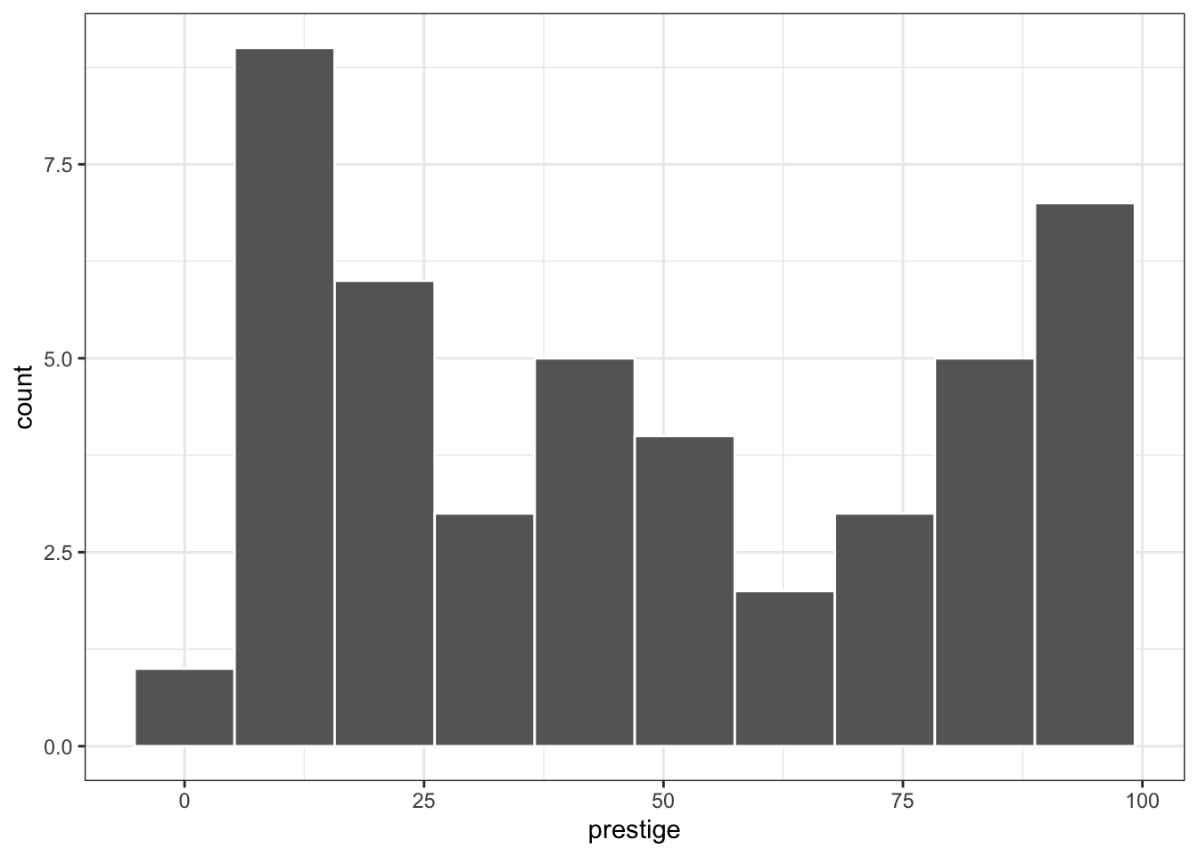
Listing / Output 1.4: Histogram of prestige variable
Code
d01.1|>ggplot2::ggplot(ggplot2::aes(x =prestige))+ggplot2::geom_histogram( bins =10, color ="white", fill ="grey40")
The distribution of prestige appears to be bimodal, with cases stacking up near the boundaries, as many occupations are either low prestige, near the lower boundary, or high prestige, near the upper boundary, with relatively fewer occupations in the middle bins of the histogram. Because prestige is a percentage, this behavior is not altogether unexpected. Variables such as this often need to be transformed, perhaps with a logit (log-odds) or similar transformation. But transforming prestige turns out to be unnecessary in this problem.
Before fitting a regression model to the data, we should also examine the distributions of the predictors education and income, along with the relationship between prestige and each predictor, and the relationship between the two predictors.
R Code 1.5 : Histogram of education variable
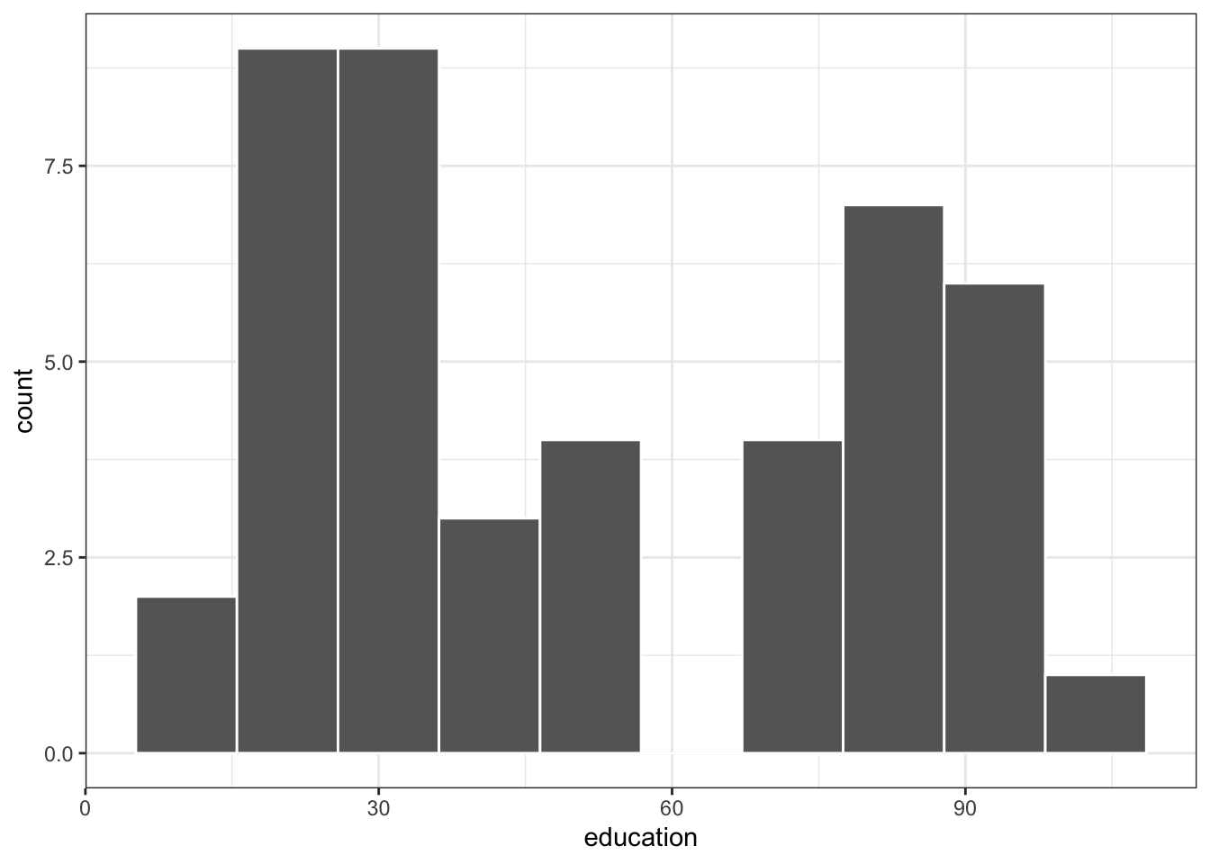
Listing / Output 1.5: Histogram of education variable
Code
d01.1|>ggplot2::ggplot(ggplot2::aes(x =education))+ggplot2::geom_histogram( bins =10, color ="white", fill ="grey40")
R Code 1.6 : Histogram of income variable
Listing / Output 1.6: Histogram of income variable
Code
d01.1|>ggplot2::ggplot(ggplot2::aes(x =income))+ggplot2::geom_histogram( bins =10, color ="white", fill ="grey40")
R Code 1.7 : Numbered R Code Title (Tidyverse)
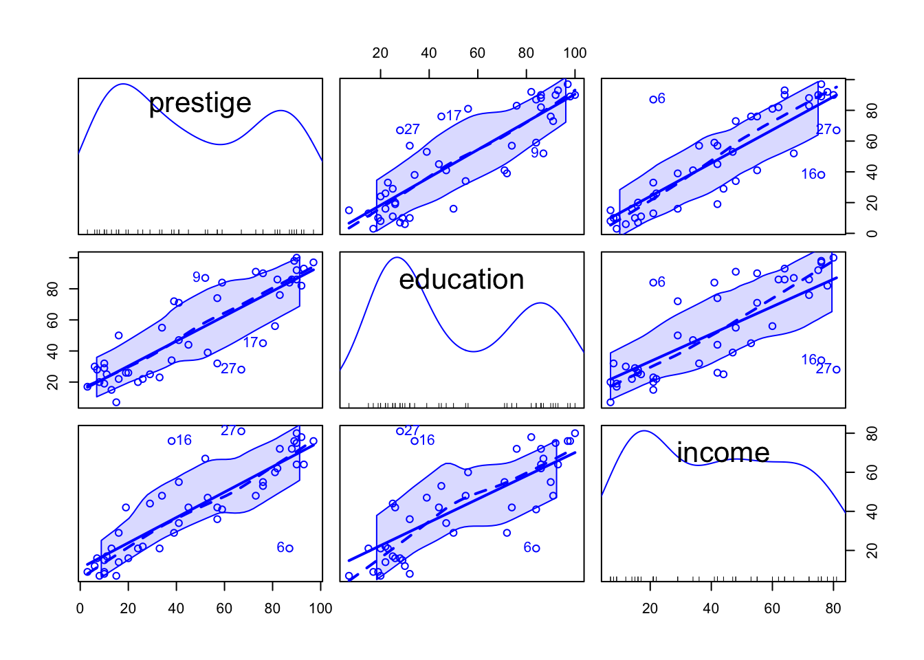
Listing / Output 1.7: Scatterplot matrix for prestige, education, and income in Duncan’s data, identifying the three most unusual points in each panel. Nonparametric density estimates for the variables appear in the diagonal panels, with a rug-plot (one-dimensional scatterplot) at the bottom of each diagonal panel.
The car::scatterplotMatrix() function uses a one-sided formula to specify the variables to appear in the graph, where we read the formula ~ prestige + education + income as “plot prestige and education and income.”
The argument id = list(n = 3) tells scatterplotMatrix() to identify the three most unusual points in each panel. This argument was added by the authors after examining a preliminary plot of the data.
Warning 1.3
In contrast to Figure 1.10 my graph shows the three most unusual points in each panel with a number and not with the name of the occupation. I believe that this difference is a result of my recoding (changing row names into a column).
Nonparametric density estimates are using an adaptive-kernel estimator, and they appear by default in the diagonal panels, with a rug-plot (“one-dimensional scatterplot”) at the bottom of each panel, showing the location of the data values for the corresponding variable.
The solid line shows the marginal linear least-squares fit for the regression of the vertical-axis variable (y) on the horizontal-axis variable (x), ignoring the other variables.
The central broken line is a nonparametric regression smooth, which traces how the average value of y changes as x changes without making strong assumptions about the form of the relationship between the two variables.
The outer broken lines represent smooths of the conditional variation of the y values given x in each panel, like running quartiles.
Note 1.1: Is there a tidyverse equivalent for car::scatterplotMatrix()?
Like prestige, education appears to have a bimodal distribution. The distribution of income, in contrast, is perhaps best characterized as irregular. The pairwise relationships among the variables seem reasonably linear, which means that as we move from left to right across the plot, the average y values of the points more or less trace out a straight line. The scatter around the regression lines appears to have reasonably constant vertical variability and to be approximately symmetric.
In addition, two or three cases stand out from the others. In the scatterplot of income versus education, data point 6 (= ministers) are unusual in combining relatively low income with a relatively high level of education, and data point 16 (= conductors) and data point 27 (= railroad engineers) are unusual in combining relatively high levels of income with relatively low education. Because education and income are predictors in Duncan’s regression, these three occupations will have relatively high leverage on the regression coefficients. None of these cases, however, are outliers in the univariate distributions of the three variables.
1.6.3 Regression Analysis
Following Duncan, we next fit a linear least-squares regression to the data to model the joint dependence of prestige on the two predictors, under the assumption that the relationship of prestige to education and income is additive and linear.
#>
#> Call:
#> stats::lm(formula = prestige ~ education + income, data = d01.1)
#>
#> Residuals:
#>     Min      1Q  Median      3Q     Max
#> -29.538  -6.417   0.655   6.605  34.641
#>
#> Coefficients:
#>             Estimate Std. Error t value Pr(>|t|)
#> (Intercept) -6.06466    4.27194  -1.420    0.163
#> education    0.54583    0.09825   5.555 1.73e-06
#> income       0.59873    0.11967   5.003 1.05e-05
#>
#> Residual standard error: 13.37 on 42 degrees of freedom
#> Multiple R-squared:  0.8282, Adjusted R-squared:   0.82
#> F-statistic: 101.2 on 2 and 42 DF,  p-value: < 2.2e-16
The “statistical-significance” asterisks were suppressed with options(show.signif.stars = FALSE).
Both education and income have large regression coefficients in the “Estimate” column of the coefficient table, with small two-sided p-values in the column labeled “Pr (>|t|)”. For example, holding education constant, a 1% increase in higher income earners is associated on average with an increase of about 0.6% in high prestige ratings.
R Code 1.10 : Nonparametric density estimate of the distribution of Studentized residuals
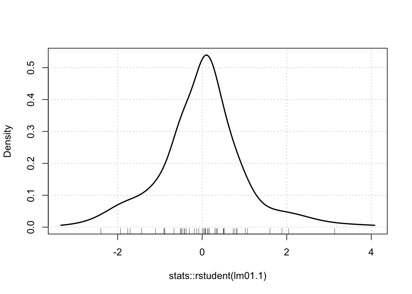
Listing / Output 1.10: Nonparametric density estimate for the distribution of the Studentized residuals from the regression of prestige on education and income.
If the errors in the regression are normally distributed with zero means and constant variance, then the Studentized residuals are each t-distributed with \(n − k − 2\) degrees of freedom, where k is the number of coefficients in the model, excluding the regression constant, and n is the number of cases.
R Code 1.11 : Quantile-comparison plot for the Studentized residuals
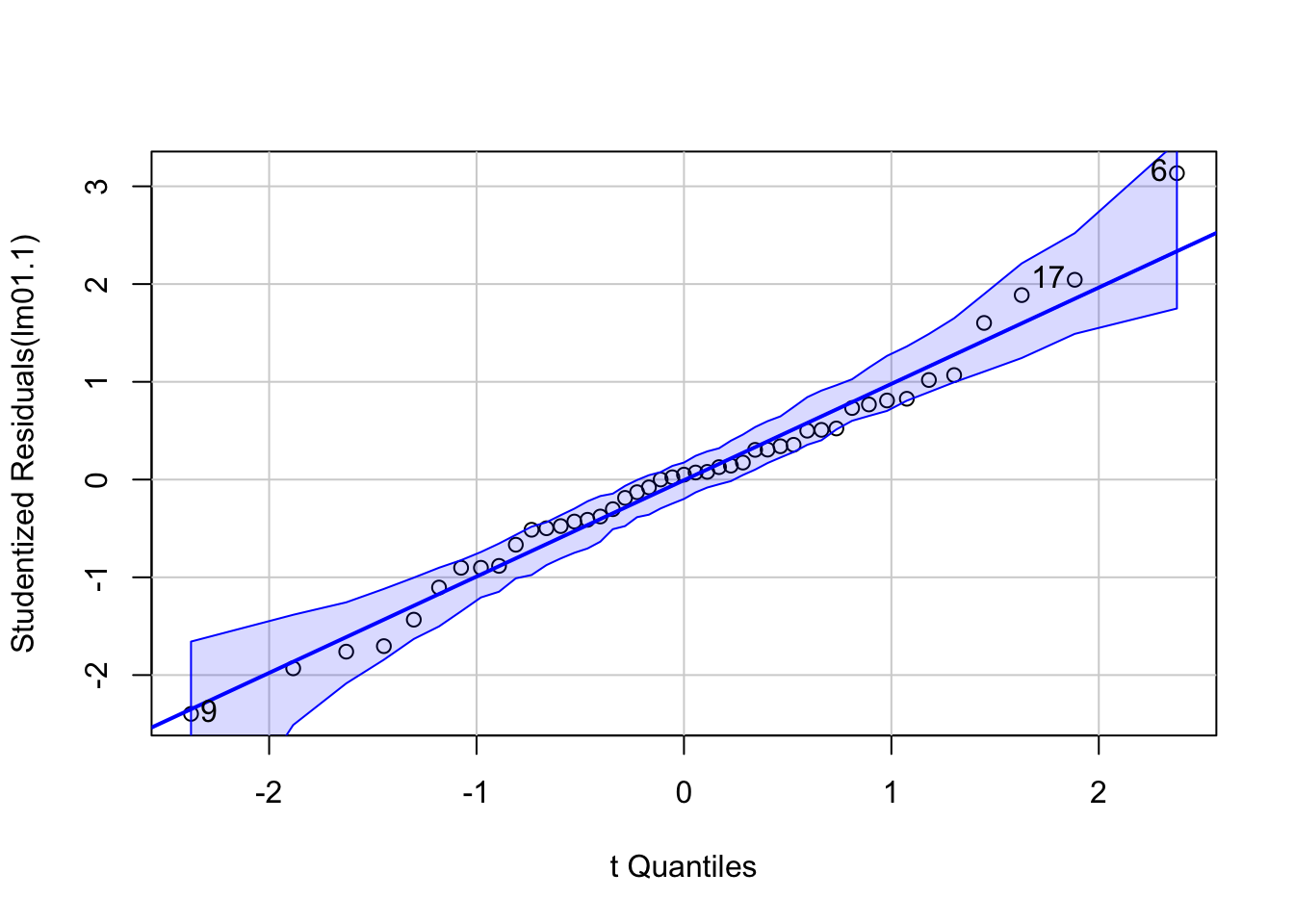
Listing / Output 1.11: Quantile-comparison plot for the Studentized residuals from the regression of prestige on education and income. The broken lines show a bootstrapped pointwise 95% confidence envelope for the points.
The car::qqPlot() function extracts the Studentized residuals and plots them against the quantiles of the appropriate t-distribution. If the Studentized residuals are t-distributed, then the plotted points should lie close to a straight line. The solid comparison line on the plot is drawn by default by robust regression. The argument id = list (n = 3) identifies the three most extreme Studentized residuals, and qqPlot() returns the (names and) row numbers of these cases.
(In my case the functions returns only the row numbers.)
6 : minister
9 : reporter
17: contractor
By default, car::qqPlot() also produces a bootstrapped pointwise 95% confidence envelope for the Studentized residuals that takes account of the correlations among them (but, because the envelope is computed pointwise, does not adjust for simultaneous inference).
Warning 1.4
Be patient! The computation of the bootstrapped pointwise 95% confidence envelope for the points takes some time.
The bootstrap procedure used by car::qqPlot() generates random samples, and so the plot that you see when you duplicate this command will not be identical to the graph shown in the text.
The residuals stay nearly within the boundaries of the envelope at both ends of the distribution, with the exception of point 6, the occupation minister.
R Code 1.12 : Test based on the largest (absolute) Studentized residual
Listing / Output 1.12: Outlier test: Studentized residuals with Bonferroni
#> No Studentized residuals with Bonferroni p < 0.05
#> Largest |rstudent|:
#>   rstudent unadjusted p-value Bonferroni p
#> 6 3.134519          0.0031772      0.14297
The outlier test suggests that the residual for ministers is not terribly unusual, with a Bonferroni-corrected p-value of 0.14.
R Code 1.13 : Checking for high-leverage and influential cases
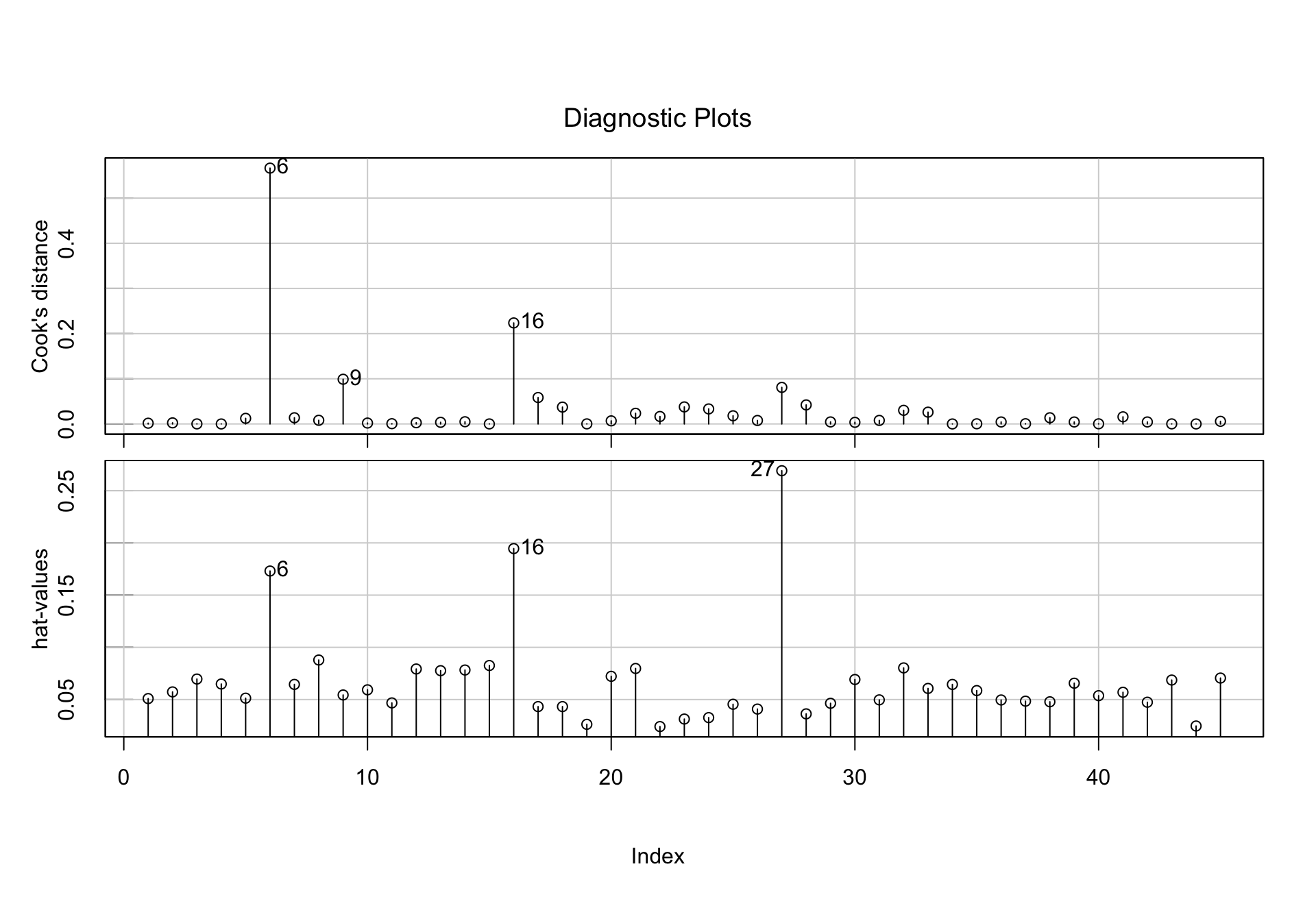
Listing / Output 1.13: Index plots of Cook’s distances and hat-values, from the regression of prestige on income and education.
Because the cases in a regression can be jointly as well as individually influential, we also examine added-variable plots for the predictors, using car::avPlots().
R Code 1.14 : Added-variable plots
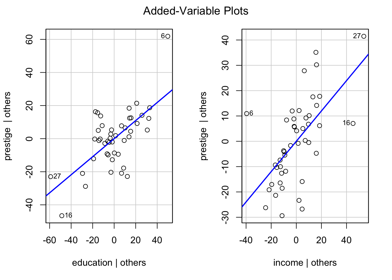
Listing / Output 1.14: Added-variable plots for education and income in Duncan’s occupational-prestige regression
Code
car::avPlots( model =lm01.1, id =list( cex =0.75, n =3, method ="mahal"))
The id argument, which has several components here, customizes identification of points in the graph:
cex = 0.75 (where cex is a standard R argument for “character expansion”) makes the labels smaller, so that they fit better into the plots
n = 3 identifies the three most unusual points in each plot
method = "mahal" indicates that unusualness is quantified by Mahalanobis distance from the center of the point-cloud.
Mahalanobis distances from the center of the data take account of the standard deviations of the variables and the correlation between them. Each added-variable plot displays the conditional, rather than the marginal, relationship between the response and one of the predictors. Points at the extreme left or right of the plot correspond to cases that have high leverage on the corresponding coefficient and consequently are potentially influential.
Listing / Output 1.14 confirms and strengthens our previous observations: We should be concerned about the occupations minister (point 6) and conductor (point 16), which work jointly to increase the education coefficient and decrease the income coefficient. Occupation RR.engineer (point 27) has relatively high leverage on these coefficients but is more in line with the rest of the data.
R Code 1.15 : Component-plus-residual plots
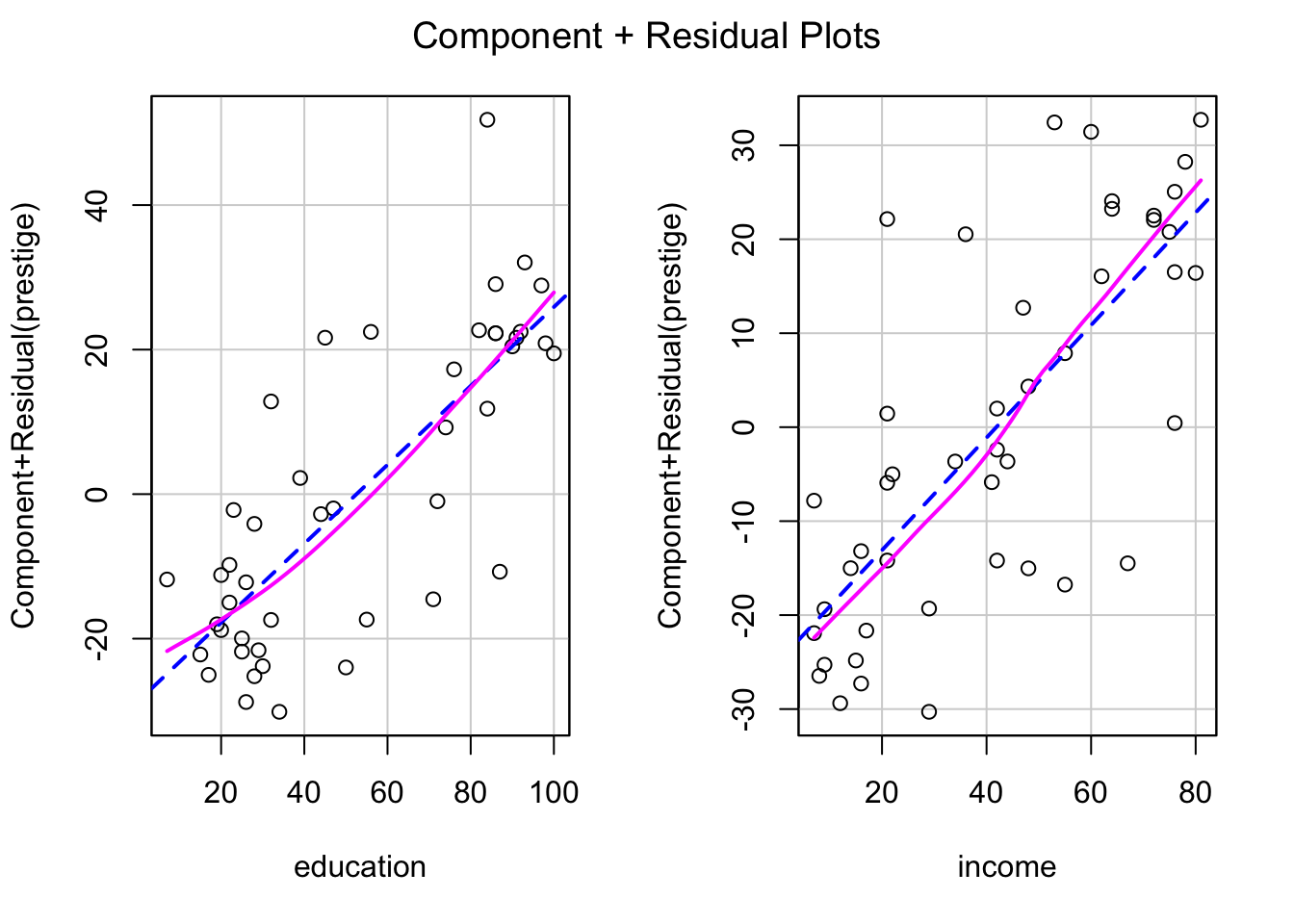
Listing / Output 1.15: Component-plus-residual plots for education and income in Duncan’s occupational-prestige regression. The solid line in each panel shows a loess nonparametric-regression smooth; the broken line in each panel is the least-squares line
Each plot includes a least-squares line, representing the regression plane viewed edge-on in the direction of the corresponding predictor, and a loess nonparametric-regression smooth.
The purpose of Listing / Output 1.15 is to detect nonlinearity, evidence of which is slightly here.
R Code 1.16 : Score tests for nonconstant variance
Listing / Output 1.16: Checking for an association of residual variability with the fitted values and with any linear combination of the predictors
Code
car::ncvTest(lm01.1)glue::glue(" ")car::ncvTest( model =lm01.1, var.formula =~income+education)
#> Non-constant Variance Score Test
#> Variance formula: ~ fitted.values
#> Chisquare = 0.3810967, Df = 1, p = 0.53702
#>
#> Non-constant Variance Score Test
#> Variance formula: ~ income + education
#> Chisquare = 0.6976023, Df = 2, p = 0.70553
Both tests yield large p-values, indicating that the assumption of constant variance is tenable
R Code 1.17 : Linear regression without influential data of 6 and 16
Listing / Output 1.17: Linear model version 2 without influential data points 6 and 16
#>
#> Call:
#> stats::lm(formula = prestige ~ education + income, data = d01.1,
#>     subset = -c(6, 16))
#>
#> Residuals:
#>     Min      1Q  Median      3Q     Max
#> -28.612  -5.898   1.937   5.616  21.551
#>
#> Coefficients:
#>             Estimate Std. Error t value Pr(>|t|)
#> (Intercept) -6.40899    3.65263  -1.755   0.0870
#> education    0.33224    0.09875   3.364   0.0017
#> income       0.86740    0.12198   7.111 1.31e-08
#>
#> Residual standard error: 11.42 on 40 degrees of freedom
#> Multiple R-squared:  0.876,  Adjusted R-squared:  0.8698
#> F-statistic: 141.3 on 2 and 40 DF,  p-value: < 2.2e-16
Rather than respecifying the regression model from scratch with stats::lm(), we refit it using the stats::update() function, removing the two potentially problematic cases via the subset argument to update().
I didn’t need car::whichNames() to get the row numbers to be removed, because I used these numbers already all the time.
R Code 1.18 : Comparing the estimated coefficients of lm01.1 and lm01.2
Listing / Output 1.18: Comparing the estimated coefficients and their standard errors across the two regressions fit to the data
#> Calls:
#> 1: stats::lm(formula = prestige ~ education + income, data = d01.1)
#> 2: stats::lm(formula = prestige ~ education + income, data = d01.1, subset =
#>    -c(6, 16))
#>
#>             Model 1 Model 2
#> (Intercept)   -6.06   -6.41
#> SE             4.27    3.65
#>
#> education    0.5458  0.3322
#> SE           0.0983  0.0987
#>
#> income        0.599   0.867
#> SE            0.120   0.122
#>
The coefficients of education and income changed substantially with the deletion of the occupations minister and conductor. The education coefficient is considerably smaller and the income coefficient considerably larger than before.
R Code 1.19 : Linear regression without influential data of 6, 9, 16, and 27
Listing / Output 1.19: Linear model version 3 without influential data points 6, 9, 16, and 27.
#> Calls:
#> 1: stats::lm(formula = prestige ~ education + income, data = d01.1, subset =
#>    -c(6, 16))
#> 2: stats::lm(formula = prestige ~ education + income, data = d01.1, subset =
#>    -c(6, 9, 16, 27))
#>
#>             Model 1 Model 2
#> (Intercept)   -6.41   -7.15
#> SE             3.65    3.41
#>
#> education    0.3322  0.3019
#> SE           0.0987  0.1121
#>
#> income        0.867   0.947
#> SE            0.122   0.142
#>
The coefficients of education and income changed not substantially with the additional deletion of the occupations reporter (9) and RR.engineer (27). The education coefficient in lm01.3 is only somewhat smaller and the income coefficient is only a little larger than with lm01.2.
1.7 R Functions for Basic Statistics (empty)
1.8 Generic Functions and Their Methods
Note 1.2: Generic function and their methods: An important explanation for me
The following text is almost completely copied from the R companion. It explains specific structures of the R language I already met in different situations but did not understand completely. This has changed now thanks to the explication in the R companion book.
Many of the most commonly used functions in R, such as summary(), print(), and plot(), produce different results depending on the arguments passed to the function. Enabling the same generic function, such as summary(), to be used for many purposes is accomplished in R through an object-oriented programming technique called object dispatch.
The details of object dispatch are implemented differently in the S3 and S4 object systems, so named because they originated in Versions 3 and 4, respectively, of the original S language on which R is based. There is yet another implementation of object dispatch in R for the more recently introduced system of reference classes (sometimes colloquially termed “R5”). Almost everything created in R is an object, such as a numeric vector, a matrix, a data frame, a linear regression model, and so on. In the S3 object system, described in this section and used for most R object-oriented programs, each object is assigned a class, and it is the class of the object that determines how generic functions process the object. We won’t take up the S4 and reference-class object systems in this book, but they too are class based and implement (albeit more complex) versions of object dispatch.
Generic functions operate on their arguments indirectly by calling specialized functions, referred to as method functions or, more compactly, as methods. Which method is invoked typically depends on the class of the first argument to the generic function.
In contrast, in the S4 object system, method dispatch can depend on the classes of more than one argument to a generic function. For example, the generic summary() function has the following definition:
The generic function summary() has one required argument, object, and the special argument ... (the ellipses) for additional arguments that could vary from one summary () method to another.
When UseMethod (“summary”) is called by the summary() generic, and the first (object) argument to summary() is of class “lm”, for example, R searches for a method function named summary.lm(), and, if it is found, executes the command summary.lm(object, ...). It is, incidentally, perfectly possible to call summary.lm() directly.
Although the generic summary() function has only one explicit argument, the method function summary.lm() has additional arguments:
Because the arguments correlation and symbolic.cor have default values (FALSE, in both cases), they need not be specified. Thus, for example, if we enter the command summary(lm01.1, correlation=TRUE), the argument correlation=TRUE is absorbed by ... in the call to the generic summary() function and then passed to the summary.lm() method, causing it to print a correlation matrix for the coefficient estimates.
R Code 1.21 : Example of the generic summary() function with additional argument
Listing / Output 1.21: Generic function summary() with additional argument
#>
#> Call:
#> stats::lm(formula = prestige ~ education + income, data = d01.1)
#>
#> Residuals:
#>     Min      1Q  Median      3Q     Max
#> -29.538  -6.417   0.655   6.605  34.641
#>
#> Coefficients:
#>             Estimate Std. Error t value Pr(>|t|)
#> (Intercept) -6.06466    4.27194  -1.420    0.163
#> education    0.54583    0.09825   5.555 1.73e-06
#> income       0.59873    0.11967   5.003 1.05e-05
#>
#> Residual standard error: 13.37 on 42 degrees of freedom
#> Multiple R-squared:  0.8282, Adjusted R-squared:   0.82
#> F-statistic: 101.2 on 2 and 42 DF,  p-value: < 2.2e-16
#>
#> Correlation of Coefficients:
#>           (Intercept) education
#> education -0.36
#> income    -0.30       -0.72
In this instance, we can call summary.lm() directly, but most method functions are hidden in (not “exported from”) the namespaces of the packages in which the methods are defined and thus cannot normally be used directly. In any event, it is good R form to use method functions only indirectly through their generics.
For example, the summary() method summary.boot(), for summarizing the results of bootstrap resampling is hidden in the namespace of the {car} package. To call this function directly to summarize an object of class “boot”, we could reference the function with the unintuitive package-qualified name car:::summary.boot(), but calling the unqualified method summary.boot() directly won’t work.
Suppose that we invoke the hypothetical generic function fun(), defined as:
fun <-  function(x, ...){
    UseMethod   ("fun")
    }
with real argument obj of class “cls”: fun (obj). If there is no method function named fun.cls(), then R looks for a method named fun.default(). For example, objects belonging to classes without summary() methods are summarized by summary.default(). If, under these circumstances, there is no method named fun.default(), then R reports an error.
We can get a listing of all currently accessible methods for the generic summary() function using the utils::methods() function, with hidden methods flagged by asterisks.
Method selection is slightly more complicated for objects whose class is a vector of more than one element. Consider, for example, an object returned by the glm() function for fitting generalized linear models (anticipating a logistic-regression example).
R Code 1.25 : List all available methods for a specific vector class
Listing / Output 1.25: List all available methods for a vectorized class
mod.mroz<-stats::glm(lfp~., family =binomial, data =Mroz)class(mod.mroz)detach("package:car", unload =TRUE)detach("package:carData", unload =TRUE)
#> [1] "glm" "lm"
The . on the right-hand side of the model formula indicates that the response variable lfp is to be regressed on all of the other variables in the Mroz data set (which is accessible because it resides in the {carData} package). If we invoke a generic function with mod.mroz as its argument, say fun(mod. mroz), then the R interpreter will look first for a method named fun.glm(). If a function by this name does not exist, then R will search next for fun.lm() and finally for fun.default(). We say that the object mod.mroz is of primary class “glm” and inherits from class “lm”.
Source Code
# Getting started with R & RStudio {#sec-chap01}```{r}#| label: setup#| results: hold#| include: falsebase::source(file ="R/helper.R")ggplot2::theme_set(ggplot2::theme_bw())options(show.signif.stars =FALSE)```## Table of content for chapter 01::::: {#obj-chap01}:::: {.my-objectives}::: {.my-objectives-header}Chapter section list:::::: {.my-objectives-container}- ~~Working with RStudio projects (empty)~~ (@sec-chap01-1)- R Basics (@sec-chap01-2)- Fixing errors and getting help (@sec-chap01-3)- ~~Organizing your work and making it reproducible (empty)~~ (@sec-chap01-4)- An Extended Illustration: Duncan's Occupational-Prestige Regression (@sec-chap01-5) - Getting, recoding and showing data (@sec-chap01-5-1) - Explorative data analysis (@sec-chap01-5-2) - Regression analysis (@sec-chap01-5-3) - Regression diagnostics (@sec-chap01-5-4)- ~~R Functions for Basic Statistics (empty)~~ (@sec-chap01-6)- Generic functions and their methods (@sec-chap01-7)::::::::::::## Working with RStudio projects (empty) {#sec-chap01-1}## R Basics {#sec-chap01-2}- A novel feature of the R help system is the facility it provides to execute most examples in the help pages via the `utils::example()` command: $$example('log')$$- A quick way to determine the arguments of an R function is to use the `args()` function:$$args('log')$$::: {.callout-warning #wrn-help-generig-functions}`args()` and `help()` functions may not be very helpful with generic functions.:::- For the full set of reserved symbols in R, see $$help('Reserved')$$- There are two types of logical operators: - vectorizes: $\&$ and $|$ vectorized resp. - single operand: $\&\&$ and $||$The unvectorized versions of the *and* (&&) and *or* (||) operators are primarily useful for writing R programs and are not appropriate for indexing vectors.## Fixing errors and getting help {#sec-chap01-3}:::{.my-bulletbox}:::: {.my-bulletbox-header}::::: {.my-bulletbox-icon}::::::::::: {#bul-getting-help}::::::: Getting help:::::::: {.my-bulletbox-body}- `base::traceback()` provides information about the sequence of function calls leading up to an error.- `utils::apropos('<searchString>')` searches for currently accessible objects whose names contain a particular character string. It returns a character vector giving the names of objects in the search list matching (as a regular expression)- `utils:find('<searchString>')` returns where objects of a given name can be found.- `??` or `help.search()` activates a broader search because it looks not only in the title fields but in other fields of the help pages as well.- `utils::RSiteSearch()` or the search engine at https://search.r-project.org/ needs an internet connection and starts a search even broader. It looks in all standard and CRAN packages, even those not installed on your system.- [CRAN task views](https://cran.r-project.org/web/views/) describe resources in R for applications in specific areas. - Views can be installed automatically via ctv::install.views("Bayesian") or ctv::update.views("Bayesian", coreOnly=TRUE) - Query information about a particular task view on CRAN from within R for example with `ctv::ctv("MachineLearning")` - Query to obtain the list of all task views available with `ctv::available.views()`- `help(package='<packageName>')` calls the index help page of an installed package in the RStudio Help tab, including the hyperlinked index of help topics documented in the package.- `r glossary("Vignette")`: - `utils::vignette()` lists available vignettes in the packages installed on your system in the code window. - `utils::browseVignettes()` open a local web page listing vignettes in the packages installed on your system - `utils::vignette(package='<packageName>')` displays the vignettes available in a particular installed package. - `vignette('vignetteName')` or vignette('<vignetteName>', package='<packageName>') opens a specific vignette.- *RStudio help*: - Menu "Help > R Help" opens an overview page with R resources - Search R help with shortcut CTRL-ALT-F1 - [Finding your way to R](https://education.rstudio.com/learn/) with three learning pathes: [Beginners](https://education.rstudio.com/learn/beginner/), [Intermediates](https://education.rstudio.com/learn/intermediate/) and [Experts](https://education.rstudio.com/learn/expert/)- *Google search*- `r glossary("StackOverflow")` and `r glossary("Cross Validated")`: - [Stack Overflow](https://stackoverflow.com/) is a question and answer site for professional and enthusiast programmers. - [Cross Validated](https://stats.stackexchange.com/) is a question and answer site for people interested in statistics, machine learning, data analysis, data mining, and data visualization.:::::::## Organizing your work and making it reproducible (empty) {#sec-chap01-4}## An Extended Illustration {#sec-chap01-5}::: {.callout-warning #wrn-chap01-illustration-not-understanding}##### Only illustration --- not yet understandingI will follow all steps of the illustration with the Duncan data set. But be aware that I am still lacking understanding of all the procedures. Hopefully these gaps will filled with the next chapters. I am planning whenever I find an explication of the routines that follow I will provide a link to cross reference illustration and explanation.:::### Getting, recoding and showing data {#sec-chap01-5-1}:::::{.my-example}:::{.my-example-header}:::::: {#exm-chap01-illustration}: Duncan's Occupational-Prestige Regression:::::::::::::{.my-example-container}::: {.panel-tabset}###### get data:::::{.my-r-code}:::{.my-r-code-header}:::::: {#cnj-chap01-show-duncan-data}: Show Duncan raw data from {**carData**} package:::::::::::::{.my-r-code-container}::: {#lst-chap01-get-duncan-data}```{r}#| label: show-duncan-datacarData::Duncan```Duncan raw data from {**carData**} package:::***The row names contains data and have to be therefore a separate column.:::::::::###### recode :::::{.my-r-code}:::{.my-r-code-header}:::::: {#cnj-chap01-recode-duncan-data}: Recode Duncan data:::::::::::::{.my-r-code-container}::: {#lst-chap01-recode-duncan-data} ```{r}#| label: recode-duncan-data#| results: hold(d01.1<- carData::Duncan |> tibble::rownames_to_column("occupation"))save_data_file("chap01", d01.1, "d01.1.rds")```Duncan data recoded:::***Duncan was interested in how `prestige` is related to `income` and `education` in combination.:::::::::###### skim data:::::{.my-r-code}:::{.my-r-code-header}:::::: {#cnj-chap01-skim-duncan}: Skim Duncan data:::::::::::::{.my-r-code-container}::: {#lst-chap01-skim-duncan}```{r}#| label: skim-duncanskimr::skim(d01.1)```Look at the recoded Duncan data::::::::::::::::::::::::### Explorative Data Analysis {#sec-chap01-5-2}Duncan used a linear least-squares regression of `prestige` on `income` and `education` to predict the prestige of occupations for which the income and educational scores were known from the U.S. Census but for which there were no direct prestige ratings. He did not use occupational type in his analysis.A sensible place to start any data analysis, including a regression analysis, is to visualize the data using a variety of graphical displays. We need the following graphs:- Univariate distributions of the three variables- Pairwise or marginal relationships among them:::::{.my-example}:::{.my-example-header}:::::: {#exm-chap01-eda}: Explorative Data Analysis (EDA) of Duncan data:::::::::::::{.my-example-container}::: {.panel-tabset}###### hist prestige:::::{.my-r-code}:::{.my-r-code-header}:::::: {#cnj-chap01-hist-prestige}: Histogram of `prestige` variable:::::::::::::{.my-r-code-container}::: {#lst-chap01-hist-prestige}```{r}#| label: hist-prestiged01.1|> ggplot2::ggplot( ggplot2::aes(x = prestige) ) + ggplot2::geom_histogram(bins =10,color ="white",fill ="grey40")```Histogram of prestige variable:::***The distribution of `prestige` appears to be bimodal, with cases stacking up near the boundaries, as many occupations are either low prestige, near the lower boundary, or high prestige, near the upper boundary, with relatively fewer occupations in the middle bins of the histogram. Because `prestige` is a percentage, this behavior is not altogether unexpected. Variables such as this often need to be transformed, perhaps with a logit (log-odds) or similar transformation. But transforming `prestige` turns out to be unnecessary in this problem.:::::::::Before fitting a regression model to the data, we should also examine the distributions of the predictors education and income, along with the relationship between prestige and each predictor, and the relationship between the two predictors.###### hist education:::::{.my-r-code}:::{.my-r-code-header}:::::: {#cnj-chap01-hist-education}: Histogram of `education` variable:::::::::::::{.my-r-code-container}::: {#lst-chap01-hist-education}```{r}#| label: hist-educationd01.1|> ggplot2::ggplot( ggplot2::aes(x = education) ) + ggplot2::geom_histogram(bins =10,color ="white",fill ="grey40")```Histogram of education variable:::***:::::::::###### hist income:::::{.my-r-code}:::{.my-r-code-header}:::::: {#cnj-chap01-hist-income}: Histogram of `income` variable:::::::::::::{.my-r-code-container}::: {#lst-chap01-hist-income}```{r}#| label: hist-incomed01.1|> ggplot2::ggplot( ggplot2::aes(x = income) ) + ggplot2::geom_histogram(bins =10,color ="white",fill ="grey40")```Histogram of income variable:::***:::::::::###### scatterplotMatrix:::::{.my-r-code}:::{.my-r-code-header}:::::: {#cnj-chap01-scatterplot-matrix}: Numbered R Code Title (Tidyverse):::::::::::::{.my-r-code-container}::: {#lst-chap01-scatterplot-matrix} ```{r}#| label: scatterplot-matrixcar::scatterplotMatrix( ~ prestige + education + income, id =list(n =3), data = d01.1)```Scatterplot matrix for prestige, education, and income in Duncan’s data, identifying the three most unusual points in each panel. Nonparametric density estimates for the variables appear in the diagonal panels, with a rug-plot (one-dimensional scatterplot) at the bottom of each diagonal panel.:::***The `car::scatterplotMatrix()` function uses a one-sided formula to specify the variables to appear in the graph, where we read the formula `~ prestige + education + income` as “plot prestige and education and income.” The argument `id = list(n = 3)` tells `scatterplotMatrix()` to identify the three most unusual points in each panel. This argument was added by the authors after examining a preliminary plot of the data.::: {.callout-warning #wrn-chap01-difference-in-scatterplot-matrix}In contrast to Figure 1.10 my graph shows the three most unusual points in each panel with a number and not with the name of the occupation. I believe that this difference is a result of my recoding (changing row names into a column).::::::::::::- **Nonparametric density estimates** are using an adaptive-kernel estimator, and they appear by default in the diagonal panels, with a *rug-plot* (“one-dimensional scatterplot”) at the bottom of each panel, showing the location of the data values for the corresponding variable.- The **solid line** shows the marginal linear least-squares fit for the regression of the vertical-axis variable (y) on the horizontal-axis variable (x), ignoring the other variables. - The **central broken line** is a nonparametric regression smooth, which traces how the average value of y changes as x changes without making strong assumptions about the form of the relationship between the two variables. - The **outer broken lines** represent smooths of the conditional variation of the y values given x in each panel, like running quartiles.::: {.callout-note #nte-chap01-spm-pairs-ggpairs}##### Is there a tidyverse equivalent for car::scatterplotMatrix()?I believe that `car::scatterplotMatrix()` is a modified `graphics::pairs()` function. `GGally::ggpairs()` is a {**ggplot2**} generalized [pairs plot matrix](https://ggobi.github.io/ggally/articles/ggpairs.html) equivalent in the tidyverse tradition. I should try it out and see if I can reproduce @lst-chap01-scatterplot-matrix with {**GGally**}.:::Like `prestige`, `education` appears to have a bimodal distribution. The distribution of `income`, in contrast, is perhaps best characterized as irregular. The pairwise relationships among the variables seem reasonably linear, which means that as we move from left to right across the plot, the average y values of the points more or less trace out a straight line. The scatter around the regression lines appears to have reasonably constant vertical variability and to be approximately symmetric.In addition, two or three cases stand out from the others. In the scatterplot of `income` versus `education`, data point 6 (= ministers) are unusual in combining relatively low income with a relatively high level of education, and data point 16 (= conductors) and data point 27 (= railroad engineers) are unusual in combining relatively high levels of income with relatively low education. Because `education` and `income` are predictors in Duncan’s regression, these three occupations will have relatively high `r glossary("leverage")` on the regression coefficients. None of these cases, however, are `r glossary("outliers")` in the *univariate* distributions of the three variables.::::::::::::### Regression Analysis {#sec-chap01-5-3}Following Duncan, we next fit a linear least-squares regression to the data to model the joint dependence of prestige on the two predictors, under the assumption that the relationship of prestige to education and income is additive and linear.:::::{.my-example}:::{.my-example-header}:::::: {#exm-chap01-ols-regression}: Compute OLS regression:::::::::::::{.my-example-container}::: {.panel-tabset}###### fit lm.1:::::{.my-r-code}:::{.my-r-code-header}:::::: {#cnj-chap01-lm-1}: Fit linear model:::::::::::::{.my-r-code-container}::: {#lst-chap01-lm-1}```{r}#| label: fit-lm1( lm01.1<- stats::lm(formula = prestige ~ education + income,data = d01.1 ))save_data_file("chap01", lm01.1, "lm01.1.rds")```Regress `prestige` on `education` and `income`::::::::::::###### summary lm.1:::::{.my-r-code}:::{.my-r-code-header}:::::: {#cnj-chap01-summary-lm-1}: Summary of lm01.1:::::::::::::{.my-r-code-container}::: {#lst-chap01-summary-lm-1} ```{r}#| label: summary-lm1base::summary(lm01.1)```Summary of linear model where `prestige` is regressed on `education` and `income`:::***The “statistical-significance” asterisks were suppressed with `options(show.signif.stars = FALSE)`.:::::::::Both education and income have large regression coefficients in the "Estimate" column of the coefficient table, with small two-sided p-values in the column labeled "Pr (>|t|)". For example, holding education constant, a 1% increase in higher income earners is associated on average with an increase of about 0.6% in high prestige ratings.::::::::::::### Regression diagnostics {#sec-chap01-5-4}:::::{.my-example}:::{.my-example-header}:::::: {#exm-chap01-regression-diagnostics}: Regression diagnostics:::::::::::::{.my-example-container}::: {.panel-tabset}###### density:::::{.my-r-code}:::{.my-r-code-header}:::::: {#cnj-chap01-density-estimate}: Nonparametric density estimate of the distribution of Studentized residuals:::::::::::::{.my-r-code-container}::: {#lst-chap01-density-estimate}```{r}#| label: density-estimatecar::densityPlot(stats::rstudent(lm01.1))```Nonparametric density estimate for the distribution of the Studentized residuals from the regression of `prestige` on `education` and `income.`:::***If the errors in the regression are normally distributed with zero means and constant variance, then the Studentized residuals are each t-distributed with $n − k − 2$ degrees of freedom, where k is the number of coefficients in the model, excluding the regression constant, and n is the number of cases.:::::::::###### qqPlot:::::{.my-r-code}:::{.my-r-code-header}:::::: {#cnj-chap01-qq-plot}: Quantile-comparison plot for the Studentized residuals:::::::::::::{.my-r-code-container}::: {#lst-chap01-qq-plot} ```{r}#| label: qq-plot#| cache: truecar::qqPlot(lm01.1, id =list(n =3))```Quantile-comparison plot for the Studentized residuals from the regression of prestige on education and income. The broken lines show a bootstrapped pointwise 95% confidence envelope for the points.:::***The `car::qqPlot()` function extracts the Studentized residuals and plots them against the quantiles of the appropriate t-distribution. If the Studentized residuals are t-distributed, then the plotted points should lie close to a straight line. The solid comparison line on the plot is drawn by default by robust regression. The argument `id = list (n = 3)` identifies the three most extreme Studentized residuals, and `qqPlot()` returns the (names and) row numbers of these cases.(In my case the functions returns only the row numbers.)- 6 : minister- 9 : reporter- 17: contractorBy default, `car::qqPlot()` also produces a bootstrapped pointwise 95% confidence envelope for the Studentized residuals that takes account of the correlations among them (but, because the envelope is computed pointwise, does not adjust for simultaneous inference).::: {.callout-warning #wrn-chap01-bootstrap-waiting-time}Be patient! The computation of the bootstrapped pointwise 95% confidence envelope for the points takes some time.The bootstrap procedure used by `car::qqPlot()` generates random samples, and so the plot that you see when you duplicate this command will not be identical to the graph shown in the text.::::::::::::The residuals stay nearly within the boundaries of the envelope at both ends of the distribution, with the exception of point 6, the occupation `minister`.###### outlierTest:::::{.my-r-code}:::{.my-r-code-header}:::::: {#cnj-chap01-outlier-test}: Test based on the largest (absolute) Studentized residual:::::::::::::{.my-r-code-container}::: {#lst-chap01-outlier-test}```{r}#| label: outlier-testcar::outlierTest(lm01.1)```Outlier test: Studentized residuals with Bonferroni:::***The outlier test suggests that the residual for ministers is not terribly unusual, with a Bonferroni-corrected p-value of 0.14.:::::::::###### influenceIndexPlot():::::{.my-r-code}:::{.my-r-code-header}:::::: {#cnj-chap01-influenctial-cases}: Checking for high-leverage and influential cases :::::::::::::{.my-r-code-container}::: {#lst-chap01-influenctial-cases}```{r}#| label: influenctial-cases#| fig-height: 7#| fig-width: 10car::influenceIndexPlot(model = lm01.1, vars =c("Cook", "hat"),id =list(n =3) )```Index plots of `r glossary("Cook’s D", "Cook’s distances")` and `r glossary("Y-hat", "hat-values")`, from the regression of `prestige` on `income` and `education.`::::::::::::Because the cases in a regression can be *jointly* as well as individually influential, we also examine *added-variable plots* for the predictors, using `car::avPlots()`.###### avPlots:::::{.my-r-code}:::{.my-r-code-header}:::::: {#cnj-chap01-av-plots}: Added-variable plots:::::::::::::{.my-r-code-container}::: {#lst-chap01-av-plots}```{r}#| label: av-plotscar::avPlots(model = lm01.1,id =list(cex =0.75,n =3,method ="mahal" ))```Added-variable plots for education and income in Duncan’s occupational-prestige regression:::***The `id` argument, which has several components here, customizes identification of points in the graph:- `cex = 0.75` (where cex is a standard R argument for “character expansion”) makes the labels smaller, so that they fit better into the plots- `n = 3` identifies the three most unusual points in each plot- `method = "mahal"` indicates that unusualness is quantified by Mahalanobis distance from the center of the point-cloud.Mahalanobis distances from the center of the data take account of the standard deviations of the variables and the correlation between them. Each added-variable plot displays the *conditional*, rather than the marginal, relationship between the response and one of the predictors. Points at the extreme left or right of the plot correspond to cases that have high leverage on the corresponding coefficient and consequently are potentially influential.:::::::::@lst-chap01-av-plots confirms and strengthens our previous observations: We should be concerned about the occupations minister (point 6) and conductor (point 16), which work jointly to increase the education coefficient and decrease the income coefficient. Occupation RR.engineer (point 27) has relatively high leverage on these coefficients but is more in line with the rest of the data.###### crPlots:::::{.my-r-code}:::{.my-r-code-header}:::::: {#cnj-chap01-cr-plots}: Component-plus-residual plots:::::::::::::{.my-r-code-container}::: {#lst-chap01-cr-plots}```{r}#| label: cr-plotscar::crPlots(lm01.1)```Component-plus-residual plots for education and income in Duncan’s occupational-prestige regression. The solid line in each panel shows a loess nonparametric-regression smooth; the broken line in each panel is the least-squares line:::***Each plot includes a least-squares line, representing the regression plane viewed edge-on in the direction of the corresponding predictor, and a loess nonparametric-regression smooth. :::::::::The purpose of @lst-chap01-cr-plots is to detect nonlinearity, evidence of which is slightly here.###### ncvTest:::::{.my-r-code}:::{.my-r-code-header}:::::: {#cnj-chap01-ncv-test}: Score tests for nonconstant variance:::::::::::::{.my-r-code-container}::: {#lst-chap01-ncv-test}```{r}#| label: ncv-test#| results: holdcar::ncvTest(lm01.1)glue::glue(" ")car::ncvTest(model = lm01.1,var.formula =~ income + education )```Checking for an association of residual variability with the fitted values and with any linear combination of the predictors:::***Both tests yield large p-values, indicating that the assumption of constant variance is tenable:::::::::###### fit-lm2:::::{.my-r-code}:::{.my-r-code-header}:::::: {#cnj-chap01-regress-lm01.2}: Linear regression without influential data of 6 and 16:::::::::::::{.my-r-code-container}::: {#lst-chap01-regress-lm01.2}```{r}#| label: regress-lm2#| results: hold d01.2<- d01.1|> dplyr::slice(-c(6, 16))lm01.2<- stats::update(lm01.1, subset =-c(6, 16))base::summary(lm01.2)save_data_file("chap01", d01.2, "d01.2.rds")save_data_file("chap01", lm01.2, "lm01.2.rds")```Linear model version 2 without influential data points 6 and 16:::***Rather than respecifying the regression model from scratch with `stats::lm()`, we refit it using the `stats::update()` function, removing the two potentially problematic cases via the subset argument to `update()`. I didn't need `car::whichNames()` to get the row numbers to be removed, because I used these numbers already all the time. :::::::::###### compareCoefs-1:::::{.my-r-code}:::{.my-r-code-header}:::::: {#cnj-chap01-compare-coefs}: Comparing the estimated coefficients of lm01.1 and lm01.2:::::::::::::{.my-r-code-container}::: {#lst-chap01-compare-coefs}```{r}#| label: compare-coefs1car::compareCoefs(lm01.1, lm01.2)```Comparing the estimated coefficients and their standard errors across the two regressions fit to the data:::***The coefficients of education and income changed substantially with the deletion of the occupations minister and conductor. The education coefficient is considerably smaller and the income coefficient considerably larger than before.:::::::::###### fit-lm3:::::{.my-r-code}:::{.my-r-code-header}:::::: {#cnj-chap01-regress-lm01.3}: Linear regression without influential data of 6, 9, 16, and 27:::::::::::::{.my-r-code-container}::: {#lst-chap01-regress-lm01.3}```{r}#| label: regress-lm3#| results: hold d01.3<- d01.1|> dplyr::slice(-c(6, 9, 16, 27))lm01.3<- stats::update(lm01.1, subset =-c(6, 9, 16, 27))base::summary(lm01.3)save_data_file("chap01", d01.3, "d01.3.rds")save_data_file("chap01", lm01.3, "lm01.3.rds")```Linear model version 3 without influential data points 6, 9, 16, and 27.::::::::::::###### compareCoefs-2:::::{.my-r-code}:::{.my-r-code-header}:::::: {#cnj-chap01-compare-coefs2}: Comparing the estimated coefficients of lm01.1 and lm01.3:::::::::::::{.my-r-code-container}::: {#lst-chap01-compare-coefs2}```{r}#| label: compare-coefs2car::compareCoefs(lm01.2, lm01.3)```Comparing the estimated coefficients and their standard errors across the two regressions fit to the data:::***The coefficients of education and income changed not substantially with the additional deletion of the occupations reporter (9) and RR.engineer (27). The education coefficient in `lm01.3` is only somewhat smaller and the income coefficient is only a little larger than with `lm01.2`.:::::::::::::::::::::## R Functions for Basic Statistics (empty) {#sec-chap01-6}## Generic Functions and Their Methods {#sec-chap01-7}::: {.callout-note #nte-chap01-generic-functions}##### Generic function and their methods: An important explanation for meThe following text is almost completely copied from the R companion. It explains specific structures of the R language I already met in different situations but did not understand completely. This has changed now thanks to the explication in the R companion book.:::Many of the most commonly used functions in R, such as `summary()`, `print()`, and `plot()`, produce different results depending on the arguments passed to the function. Enabling the same *generic function*, such as `summary()`, to be used for many purposes is accomplished in R through an *object-oriented programming technique* called *object dispatch*.The details of object dispatch are implemented differently in the S3 and S4 object systems, so named because they originated in Versions 3 and 4, respectively, of the original S language on which R is based. There is yet another implementation of object dispatch in R for the more recently introduced system of reference classes (sometimes colloquially termed “R5”). Almost everything created in R is an object, such as a numeric vector, a matrix, a data frame, a linear regression model, and so on. In the S3 object system, described in this section and used for most R object-oriented programs, each object is assigned a class, and it is the class of the object that determines how generic functions process the object. We won’t take up the S4 and reference-class object systems in this book, but they too are class based and implement (albeit more complex) versions of object dispatch.Generic functions operate on their arguments indirectly by calling specialized functions, referred to as method functions or, more compactly, as methods. Which method is invoked typically depends on the class of the first argument to the generic function.In contrast, in the S4 object system, method dispatch can depend on the classes of more than one argument to a generic function. For example, the generic `summary()` function has the following definition: ```- **summary** - function (object, ...) - UseMethod ("summary") -<bytecode: 0x000000001d03ba78> - <environment: namespace:base> ```The generic function `summary()` has one required argument, object, and the special argument `...` (the ellipses) for additional arguments that could vary from one `summary ()` method to another.When UseMethod ("summary") is called by the `summary()` generic, and the first (object) argument to `summary()` is of class "lm", for example, R searches for a method function named `summary.lm()`, and, if it is found, executes the command `summary.lm(object, ...)`. It is, incidentally, perfectly possible to call `summary.lm()` directly.Although the generic `summary()` function has only one explicit argument, the method function `summary.lm()` has additional arguments: ```- args("summary.lm") - function(object, correlation = FALSE, symbolic.cor = FALSE, ...) - NULL```Because the arguments `correlation` and `symbolic.cor` have default values (FALSE, in both cases), they need not be specified. Thus, for example, if we enter the command `summary(lm01.1, correlation=TRUE)`, the argument `correlation=TRUE` is absorbed by `...` in the call to the generic `summary()` function and then passed to the `summary.lm()` method, causing it to print a correlation matrix for the coefficient estimates.:::::{.my-r-code}:::{.my-r-code-header}:::::: {#cnj-chap01-generic-function-additional-argument}: Example of the generic `summary()` function with additional argument:::::::::::::{.my-r-code-container}::: {#lst-chap01-generic-function-additional-argument}```{r}#| label: generic-function-additional-argumentsummary.lm(lm01.1, correlation =TRUE)```Generic function `summary()` with additional argument::::::::::::In this instance, we can call `summary.lm()` directly, but most method functions are hidden in (not “exported from”) the namespaces of the packages in which the methods are defined and thus cannot normally be used directly. In any event, it is good R form to use method functions only indirectly through their generics. For example, the `summary()` method `summary.boot()`, for summarizing the results of bootstrap resampling is hidden in the namespace of the {**car**} package. To call this function directly to summarize an object of class "boot", we could reference the function with the unintuitive package-qualified name `car:::summary.boot()`, but calling the unqualified method `summary.boot()` directly won’t work.Suppose that we invoke the hypothetical generic function `fun()`, defined as: ```fun <- function(x, ...){ UseMethod ("fun") } ```with real argument obj of class "cls": `fun (obj)`. If there is no method function named `fun.cls()`, then R looks for a method named `fun.default()`. For example, objects belonging to classes without `summary()` methods are summarized by `summary.default()`. If, under these circumstances, there is no method named `fun.default()`, then R reports an error.We can get a listing of all currently accessible methods for the generic `summary()` function using the `utils::methods()` function, with hidden methods flagged by asterisks.:::::{.my-example}:::{.my-example-header}:::::: {#exm-chap01-generic-functions}: Generic functions and their methods:::::::::::::{.my-example-container}::: {.panel-tabset}###### methods1:::::{.my-r-code}:::{.my-r-code-header}:::::: {#cnj-chap01-list-methods}: Listing for all the methods for a generic function:::::::::::::{.my-r-code-container}::: {#lst-chap01-list-methods}```{r}#| label: list-methodsutils::methods(summary)```List all the methods for the generic function `summary()`::::::::::::You can also determine what generic functions have currently available methods for objects of a particular class.###### methods-class1:::::{.my-r-code}:::{.my-r-code-header}:::::: {#cnj-chap01-list-class-methods}: List all available methods for a specific class:::::::::::::{.my-r-code-container}::: {#lst-chap01-list-class-methods} ```{r}#| label: list-class-methodsutils::methods(class ="lm")```List all available methods for a class = "lm"::::::::::::In the above code chunk I have not loaded the {**car**} package which has many other methods for class "lm". (See next tab)###### methods-class2:::::{.my-r-code}:::{.my-r-code-header}:::::: {#cnj-chap01-list-class-methods2}: List all available methods for a specific class with additional package loaded:::::::::::::{.my-r-code-container}::: {#lst-chap01-list-class-methods2}```{r}#| label: list-class-methods2#| results: holdlibrary(car)utils::methods(class ="lm")detach("package:car", unload =TRUE)detach("package:carData", unload =TRUE)```Example of using the `methods()` function with the {**car**} package loaded::::::::::::Method selection is slightly more complicated for objects whose class is a vector of more than one element. Consider, for example, an object returned by the `glm()` function for fitting generalized linear models (anticipating a logistic-regression example).###### methods-class3:::::{.my-r-code}:::{.my-r-code-header}:::::: {#cnj-chap01-list-class-methods3}: List all available methods for a specific vector class:::::::::::::{.my-r-code-container}::: {#lst-chap01-list-class-methods3}```{r}#| label: list-class-methods3#| results: holdlibrary(car)mod.mroz <- stats::glm( lfp ~ ., family = binomial, data = Mroz)class(mod.mroz)detach("package:car", unload =TRUE)detach("package:carData", unload =TRUE)```List all available methods for a vectorized class ::::::::::::The `.` on the right-hand side of the model formula indicates that the response variable `lfp` is to be regressed on all of the other variables in the `Mroz` data set (which is accessible because it resides in the {**carData**} package). If we invoke a generic function with `mod.mroz` as its argument, say `fun(mod. mroz)`, then the R interpreter will look first for a method named `fun.glm()`. If a function by this name does not exist, then R will search next for `fun.lm()` and finally for `fun.default()`. We say that the object `mod.mroz` is of *primary class* "glm" and *inherits* from class "lm".::::::::::::