Chapter 3 Stratification

3.1 What is it?

Stratification is a commonly used technique in survey sampling, which consists of dividing the target population \(U\) into \(H\) non overlapping sub-populations \(U_1, U_2 \cdots U_H\), called strata, which comprise the whole population \(U\).

A sample \(s_h\) of size \(n_h\) is taken within each stratum \(h\) independently from one stratum to another. Let \(n = \sum_{h=1}^H n_h\) denote the overall sample size.

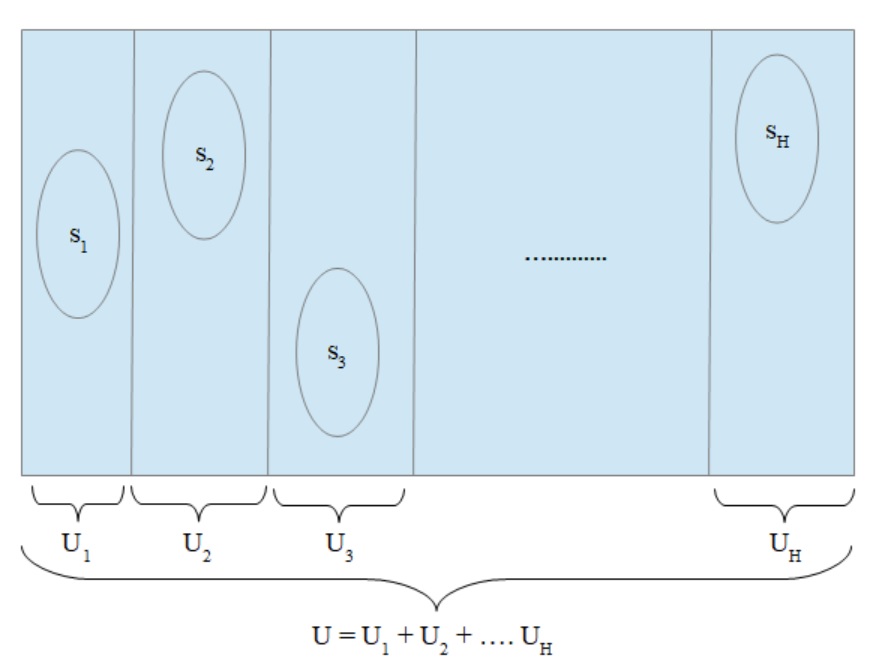
Figure 3.1: Stratification

For example, we can divide a population of individuals according to the age and the gender of the person or its city of residence. As to a population of businesses, it can be stratified by characteristics such as company size or sector of activity as set out by the NACE classification.

Stratification provides an example of a sampling technique whereby auxiliary information is mobilized in order to improve sampling efficiency. This auxiliary information is given by stratification characteristics whose values are assumed to be known a priori for every unit in the target population. As we’ll see, stratification will make data accuracy better when the stratification variables used are well related to the study variables of the survey.

Overall, stratification is driven either by statistical considerations (the need to get more accurate results at global or local level) or by organisational aspects (a stratum corresponds to a “regional” office which is in charge of data collection within the region)

3.2 Total, mean and proportion estimators

Let \(N_h\) be the size of stratum \(h\). In stratification, the size \(N_h\) is assumed to be known for all strata \(h\). In which case, the total \(Y\) of a study variable \(y\) can be written as:

\[\begin{equation} Y = \sum_{i \in U} y_i = \sum_{h=1}^{H} \sum_{i \in U_h} y_i = \sum_{h=1}^{H} Y_h = \sum_{h=1}^{H} N_h \bar{Y}_h \tag{3.1} \end{equation}\]

As to the population mean \(\bar{Y}\) of \(y\), it can be written as the average of the stratum means \(\bar{Y}_h\) using the ratios \(W_h = N_h/N\) as weights:

\[\begin{equation} \bar{Y} = \sum_{h=1}^{H} \frac{N_h}{N} \bar{Y}_h = \sum_{h=1}^{H} W_h \bar{Y}_h \tag{3.2} \end{equation}\]

Similarly, the proportion \(P\) is written as a weighted function of the stratum proportions \(P_h\):

\[\begin{equation} P = \sum_{h=1}^{H} \frac{N_h}{N} P_h = \sum_{h=1}^{H} W_h P_h \tag{3.3} \end{equation}\]

Assuming simple random sampling within each stratum (stratified simple random sampling), unbiased estimators of population totals, means and proportions are given by:

\[\begin{equation} \hat{Y}_{STSRS} = \sum_{h=1}^{H} N_h \bar{y}_h \tag{3.4} \end{equation}\]

\[\begin{equation} \hat{\bar{Y}}_{STSRS} = \sum_{h=1}^{H} W_h \bar{y}_h \tag{3.5} \end{equation}\]

\[\begin{equation} \hat{P}_{STSRS} = \sum_{h=1}^{H} W_h p_h \tag{3.6} \end{equation}\]

In stratified simple random sampling, the design weights are equal within each stratum: \(d_i = N_h/n_h ~~\forall i \in s_h\)

Using the results for simple random sampling, the variances of the three above estimators are given by:

\[\begin{equation} V\left(\hat{Y}_{STSRS}\right) = \sum_{h=1}^{H} N^2_h \left(1-f_h\right) S^2_h / n_h \tag{3.7} \end{equation}\]

\[\begin{equation} V\left(\hat{\bar{Y}}_{STSRS}\right) = \sum_{h=1}^{H} W^2_h \left(1-f_h\right) S^2_h / n_h \tag{3.8} \end{equation}\]

\[\begin{equation} V\left(\hat{P}_{STSRS}\right) \approx \sum_{h=1}^{H} W^2_h \left(1-f_h\right) P_h\left(1-P_h\right) / n_h \tag{3.9} \end{equation}\]

Assuming the sampling fraction \(f_h\) is the same in each stratum: \(f_h = n_h/N_h = n/N = f ~~\forall h\), we can then rewrite the estimator (3.8) as:

\[\begin{equation} \begin{array}{rcl} V\left(\hat{\bar{Y}}_{STSRS}\right) & = & \sum_{h=1}^{H} W^2_h \left(1-f_h\right) S^2_h / n_h \\ & = & \left(1-f\right) \sum_{h=1}^{H} W^2_h S^2_h / n_h \\ & = & \left(1-f\right) \sum_{h=1}^{H} W_h S^2_h / n \\ & = & \left(1-f\right) S^2_w / n \end{array} \tag{3.10} \end{equation}\]

where \(S^2_w = \sum_{h=1}^{H} W_h S^2_h\) is the within-stratum dispersion.

As \(S^2_w\) is lower than the total population dispersion \(S^2\), it can be shown that:

\[ V\left(\hat{\bar{Y}}_{STSRS}\right) = \left(1-f\right) S^2_w / n \leq \left(1-f\right) S^2 / n = V\left(\hat{\bar{Y}}_{SRS}\right) \] Therefore, stratification leads to mean estimators which are more accurate than those obtained under simple random sampling. The gain in accuracy is directly measured through the ratio \(\rho = S^2_w / S^2\): the more homegeneous the stratum groups with respect to the study variable, the better the gain. For instance, in a survey about housing rents, stratification should be done according to characteristics such as geographical region, dwelling type or living area. In a business survey, relevant stratification criteria are company size or sector of activity (NACE)

3.3 Sample allocation

Let assume the overall sample size \(n\) has been fixed (generally out of budgetary considerations). We seek to determine which sample size \(n_h\) is to be drawn out of each stratum in order to achieve statistical optimality under cost considerations. To that end, different allocation schemes have been proposed in the literature.

3.3.1 Equal allocation

In equal allocation, the sample size \(n_h\) is constant across the stratum groups: \[\begin{equation} \forall h~~n^{eq}_h=n/H \tag{3.11} \end{equation}\]

This scheme ensures a minimum level of precision in each stratum. It is therefore driven by local considerations. On the other hand, equal allocation performs poorly when it comes to national estimation, especially when the dispersions \(S^2_h\) are different from one stratum to another.

3.3.2 Proportional allocation

Proportional allocation consists of selecting samples in each stratum in proportion to the size \(N_h\) of the stratum population: \[\begin{equation} \forall h~~n^{prop}_h = n N_h / N = nW_h \tag{3.12} \end{equation}\]

As previously shown, proportional allocation is always more efficient in terms of sample accuracy than simple random sampling of same size \(n\).

\[\begin{equation} V\left(\hat{\bar{Y}}_{prop}\right) = \left(1-f\right)\frac{S^2_w}{n} = \frac{\sum_{h=1}^{H} W_h S^2_h}{n} - \frac{\sum_{h=1}^{H} W_h S^2_h}{N} \tag{3.13} \end{equation}\]

This result justifies the use of stratification as a powerful variance reduction technique.

3.3.3 Optimal allocation

Optimal allocation (also called Neyman allocation) seeks to minimize the variance (3.8) under the cost constraint \(\sum_{h=1}^H c_h n_h = C_0\), where \(C_0\) is the overall budget available and \(c_h\) the average survey cost for an individual in stratum \(h\).

The solution to this problem is given by: \[\begin{equation} \forall h~~n^{opt}_h = \frac{N_h S_h}{\sqrt{c_h}} \frac{C_0}{\sum_{h=1}^H N_h S_h \sqrt{c_h}} \tag{3.14} \end{equation}\]

If there is no cost constraint across the strata (i.e. \(c_h=1~~\forall h\)), then the sample size in stratum \(h\) is: \[\begin{equation} n^{opt}_h = n \frac{N_h S_h}{\sum_{h=1}^H N_h S_h} \tag{3.15} \end{equation}\]

and the variance of (3.8) under Neyman allocation (3.15) is:

\[\begin{equation} \begin{array}{rcl} V\left(\hat{\bar{Y}}_{opt}\right) & = & \displaystyle{\frac{\left(\sum_{h=1}^{H} W_h S_h\right)^2}{n} - \frac{\sum_{h=1}^{H} W_h S^2_h}{N}} \\ & = & \displaystyle{V\left(\hat{\bar{Y}}_{prop}\right) - \frac{1}{n} \sum_h W_h \left(S_h - \bar{S}\right)^2} \\ & = & \displaystyle{V\left(\hat{\bar{Y}}_{SRS}\right) - \frac{1}{n} \sum_h W_h \left(\bar{Y}_h - \bar{Y}\right)^2 - \frac{1}{n} \sum_h W_h \left(S_h - \bar{S}\right)^2} \tag{3.16} \end{array} \end{equation}\]

Contrary to proportional allocation, the Neyman allocation is variable-specific: optimality is defined with respect to one study variable, and what is optimal with respect to one variable may be far from optimal with respect to another.

In addition, one can prove (see e.g. Cochran (1977)) the gain in accuracy as compared to proportional allocation is pretty small. That’s why in practice proportional allocation is often preferred to optimal allocation.

3.3.4 Balanced allocation

Both proportional and Neyman allocations increase sample accuracy at global level, but may happen to perform very poorly when it comes to regional level estimates. For instance, proportional allocation of a global sample of 5000 individuals would lead to a sample of 500 individuals when the stratum weight \(W_h\) is equal to 10% of the whole population, and only 100 individuals when the weight is equal to 2%.

In order to reconcile local and global considerations, a balanced approach can be adopted: a subsample \(\tilde{n} \leq n\) may be equally allocated among the strata in order to ensure a minimum level of precision in each group, while the rest of the sample, of size \(n - \tilde{n}\), may be allocated using either proportional or optimal allocations in order to optimize accuracy at global level.

\[\begin{equation} \forall h~~n^{bal}_h = \displaystyle{\frac{\tilde{n}}{H}} + \left(n-\tilde{n}\right) W_h \tag{3.17} \end{equation}\]

As a conclusion, we can say that stratification is a well established technique which serves both for statistical and organisational purposes. That’s why it is so commonly used in survey practice, especially by National Statistical Institutes such as STATEC.