Chapter 2 Simple random sampling

2.1 Definition

Simple random sampling (SRS) is a method of selecting n units out of N such that every sample s of size n has the same probability of selection:

\[\begin{equation} Pr\left(S=s\right) = 1 / \binom{N}{n} \tag{2.1} \end{equation}\]

Where \(\binom{N}{n}\) denotes the total number of samples of size \(n\) out of \(N\) units.

Basically, this is what is done when \(n\) balls are selected in a lottery:

• First draw: one unit is selected with probability \(1/N\)
• Second draw: one unit is selected with probability \(1/N-1\) …
• \(n^{th}\) draw: one unit is selected with probability \(1/N-(n-1)\)

Thus the probability of selection of \(s \in \mathcal{S}\) is given by:

\[\begin{equation} \begin{array}{lcl} Pr\left(S=s\right) & = & n! \times \frac{1}{N} \times \frac{1}{N} \times \cdots \frac{1}{N-(n-1)} \\ & = & n! \times \frac{(N-n)!}{N!} \\ & = & 1 / \binom{N}{n} \\ \end{array} \tag{2.2} \end{equation}\]

Simple random sampling is the most basic form of sampling scheme, requiring no auxiliary information to be implemented.

2.2 Inclusion probabilities

Inclusion probabilities are key notions in survey sampling. Basically, they are defined by the probability for a unit (simple inclusion probability) or a couple of units (double inclusion probability) to appear in the sample.

The simple inclusion probability of \(i \in U\) is given by:

\[\begin{equation} \pi_{i} = Pr\left(i \in S\right) = \sum_{\substack {s \in \mathcal{S} \\ s \ni i}} Pr\left(S = s\right) = \frac{\binom{N-1}{n-1}}{\binom{N}{n}} = \frac{n}{N} \tag{2.3} \end{equation}\]

The double inclusion probability of \(i\) and \(j \in U\) \(\left(i \neq j\right)\) is given by:

\[\begin{equation} \pi_{ij} = Pr\left(i,j \in S\right) = \sum_{\substack {s \in \mathcal{S} \\ s \ni i,j}} Pr\left(S = s\right) = \frac{\binom{N-2}{n-2}}{\binom{N}{n}} = \frac{n}{N} \frac{n-1}{N-1} \tag{2.4} \end{equation}\]

2.3 Estimating population totals and means

Suppose we wish to estimate the total \(Y\) of a study variable \(y\) over the target population \(U\): \[\begin{equation} Y = \sum_{k \in U} y_k \tag{2.5} \end{equation}\]

Assuming the size \(N\) of the population is known, the mean of a variable can be regarded as a particular case of a total: \[\begin{equation} \bar{Y} = (1/N) \sum_{k \in U} y_k = \sum_{k \in U} \left(y_k / N\right) = \sum_{k \in U} z_k \tag{2.6} \end{equation}\]

In the absence of any additional information, we are going to use the following estimator of \(\bar{Y}\): \[\begin{equation} \hat{\bar{Y}}_{SRS} = \bar{y} \tag{2.7} \end{equation}\]

Hence the population total \(Y = N\bar{Y}\) is estimated by: \[\begin{equation} \hat{Y}_{SRS} = N\bar{y} \tag{2.8} \end{equation}\]

Result 1: The sample mean \(\bar{y}\) is an unbiased estimator of the population mean \(\bar{Y}\)

We have: \(E\left(\bar{y}\right) = \sum_{s \in \mathcal S} Pr\left(S=s\right) \displaystyle{\frac{\sum_{i \in s} y_i}{n}} = \displaystyle{\frac{1}{n\binom{N}{n}}}\sum_{s \in \mathcal S} \displaystyle{\sum_{i \in s} y_i}= \displaystyle{\frac{\binom{N-1}{n-1}}{n\binom{N}{n}}}\displaystyle{\sum_{i \in U} y_i} = \bar{Y}\)

Result 2: The variance of \(\bar{y}\) is given by: \[\begin{equation} V\left(\bar{y}\right) = \left(1-\frac{n}{N}\right)\frac{S^2_y}{n} = \left(1-f\right)\frac{S^2_y}{n} \tag{2.9} \end{equation}\]

where

• \(S^2_y\) is the dispersion of the study variable \(y\) over the population \(U\): \(S^2_y = \frac{1}{N-1}\sum_{i \in U} \left(y_i - \bar{Y}\right)^2\)
• \(f=n/N\) is the sampling rate or sampling fraction
• \(1-f\) is called the finite population correction factor

Proof: We have: \(E\left(\bar{y}^2\right) = \sum_{s \in \mathcal S} Pr\left(S=s\right) \displaystyle{\left(\frac{\sum_{i \in s} y_i}{n}\right)^2} = \displaystyle{\frac{1}{n^2\binom{N}{n}}}\sum_{s \in \mathcal S} \displaystyle{\left(\sum_{i \in s} y_i\right)^2}\)

\(= \displaystyle{\frac{1}{n^2\binom{N}{n}}}\sum_{s \in \mathcal S} \displaystyle{\sum_{i \in s} y^2_i}+ \displaystyle{\frac{1}{n^2\binom{N}{n}}}\sum_{s \in \mathcal S} \displaystyle{\sum_{i \in s , j \in s j \neq i} y_i y_j}\)

\(= \displaystyle{\frac{\binom{N-1}{n-1}}{n^2\binom{N}{n}}}\displaystyle{\sum_{i \in U} y^2_i}+ \displaystyle{\frac{\binom{N-2}{n-2}}{n^2\binom{N}{n}}} \displaystyle{\sum_{i \in U , j \in U j \neq i} y_i y_j}\)

\(= \displaystyle{\frac{1}{nN}}\displaystyle{\sum_{i \in U} y^2_i}+ \displaystyle{\frac{\left(n-1\right)}{nN\left(N-1\right)}} \left[ \displaystyle{\left(\sum_{i \in U} y_i\right)^2 - \sum_{i \in U} y^2_i} \right]\)

\(= \displaystyle{\frac{1}{nN}\frac{N-n}{N-1}}\displaystyle{\sum_{i \in U} y^2_i} + \displaystyle{\frac{N\left(n-1\right)}{n\left(N-1\right)}\bar{Y}^2}\)

Hence the variance of \(\bar{y}\) is given by:

\(V\left(\bar{y}\right) = E\left(\bar{y}^2\right) - \bar{Y}^2 = \displaystyle{\frac{1}{nN}\frac{N-n}{N-1}}\displaystyle{\sum_{i \in U} y^2_i} - \displaystyle{\frac{N-n}{n\left(N-1\right)}\bar{Y}^2}\)

\(=\displaystyle{\frac{1}{n}\frac{N-n}{N-1}\left(\frac{1}{N}\sum_{i \in U} y^2_i - \bar{Y}^2\right) = \frac{1}{n}\frac{N-n}{N}S^2_y = \frac{1-f}{n}S^2_y}\)

Result 3: The variance of the estimator \(\hat{Y}_{SRS} = N\bar{y}\) is given by: \[\begin{equation} V\left(\hat{Y}_{SRS}\right) = N^2\left(1-f\right)\frac{S^2_y}{n} \tag{2.10} \end{equation}\]

Result 4: An unbiased estimator for the variance is given by: \[\begin{equation} \hat{V}\left(\bar{y}\right) = \left(1-f\right)\frac{s^2_y}{n} \tag{2.11} \end{equation}\]

where \(s^2_y\) is the dispersion of the study variable \(y\) over the sample: \(s^2_y = \frac{1}{n-1}\sum_{i \in s} \left(y_i - \bar{y}\right)^2\).

Proof: Through expanding the sample dispersion, we have: \[\begin{equation} \begin{array}{rcl} s^2_y & = & \displaystyle{\frac{1}{n-1}\sum_{i \in s} \left(y_i - \bar{y}\right)^2} \\ & = & \displaystyle{\frac{1}{n-1}\sum_{i \in s} \left(y^2_i - 2 y_i \bar{y} + \bar{y}^2\right)} \\ & = & \displaystyle{\frac{1}{n-1}\sum_{i \in s} y^2_i} - 2 \displaystyle{\frac{1}{n-1} \left(\sum_{i \in s} y_i\right) \bar{y}} + \displaystyle{\frac{n}{n-1}\bar{y}^2} \\ & = & \displaystyle{\frac{n}{n-1}\frac{1}{n}\sum_{i \in s} y^2_i} - \displaystyle{\frac{n}{n-1}\bar{y}^2} \end{array} \end{equation}\]

By taking the expectation, we have:

\[\begin{equation} \begin{array}{rcl} E\left(s^2_y\right) & = & \displaystyle{\frac{n}{n-1}\frac{1}{N}\sum_{i \in U} y^2_i} - \displaystyle{\frac{n}{n-1}E\left(\bar{y}^2\right)} \\ & = & \displaystyle{\frac{n}{n-1}\frac{1}{N}\sum_{i \in U} y^2_i} - \displaystyle{\frac{n}{n-1}\left[V\left(\bar{y}\right) + E^2\left(\bar{y}\right) \right]} \\ & = & \displaystyle{\frac{n}{n-1}\left(\frac{1}{N}\sum_{i \in U} y^2_i - \bar{Y}^2\right)}- \displaystyle{\frac{n}{n-1}\left[\left(1-f\right)\frac{S_y^2}{n}\right]} \\ & = & \displaystyle{\frac{n}{n-1}\frac{N-1}{N}S_y^2} - \displaystyle{\frac{n}{n-1}\left[\left(1-f\right)\frac{S_y^2}{n}\right]} \\ & = & \displaystyle{S_y^2~\frac{n}{n-1}\left[\frac{N-1}{N}-\left(1-f\right)\frac{1}{n}\right]} \\ & = & \displaystyle{S_y^2~\frac{n}{n-1}\left[\frac{N-1}{N}-\frac{N-n}{Nn}\right]} = S^2_y \end{array} \end{equation}\]

The main lessons to be drawn from (2.9), (2.10) and (2.11) are the following:

• The variance is directly related to the size \(n\) of the sample: the higher the size, the lower the variance
• The variance depends on the dispersion \(S^2_y\) of the study variable: assuming the sample size is fixed, the lower the dispersion \(S^2_y\), the lower the variance
• The impact of the population size \(N\) on variance is often negligible. Basically, this means surveying 1,000 individuals from a population of 500,000 leads to results which are as accurate as when we survey 1,000 individuals from a population of 100,000,000. Put another way, sample precision is influenced by the sample size \(n\) and not the sampling rate \(n/N\).

2.4 Estimating population counts and proportions

A common population parameter one may wish to estimate from a sample survey is the size of a sub-population of interest. For instance, we seek to estimate the total number of males or females in the population, the number of elderly people aged more than 65 or the total number of establishments having more than 50 employees in a certain geographical region or in a sector of activity.

Through introducing dummy membership variables the size \(N_A\) of a subpopulation \(U_A \subseteq U\) is a particular example of a population total over the population \(U\) and, assuming the size \(N\) of the whole population is known, the proportion \(P_A = N_A/N\) is a particular case of a mean:

• \(N_A = \sum_{k \in U_A} 1 = \sum_{k \in U} 1^A_k\)
• \(P_A = \left(1/N\right) \sum_{k \in U_A} 1 = \sum_{k \in U} \left(1^A_k / N\right)\)

Hence, we obtain the following results:

Result 1: The size \(N_A\) of \(U_A\) is estimated by: \[\begin{equation} \hat{N}_A = N p_A \tag{2.12} \end{equation}\]

where \(p_A\) is the sample proportion of units from \(U_A\)

Result 2: Assuming the size \(N\) of the population is large enough and the sampling fraction is close to 0, the variance of the estimator \(N p_A\) is given by:

\[\begin{equation} \begin{array}{lcl} V\left(N p_A\right) & = & N^2\left(1-f\right){\displaystyle \frac{N}{N-1}} {\displaystyle \frac{P_A\left(1-P_A\right)}{n}} \\ & \approx & N^2{\displaystyle \frac{P_A\left(1-P_A\right)}{n}} \\ \end{array} \tag{2.13} \end{equation}\]

Proof: The dispersion of the dummy variable \(1^A\) is given by: \[\begin{equation} \begin{array}{rcl} S^2 & = & \displaystyle{\frac{1}{N-1} \sum_{i \in U} \left(1_i^A - P_A\right)^2} \\ & = & \displaystyle{\frac{1}{N-1} \left[\sum_{i \in U_A} \left(1 - P_A\right)^2 +\sum_{i \notin U_A} \left(0 - P_A\right)^2 \right]} \\ & = & \displaystyle{\frac{1}{N-1} \left[ NP_A\left(1 - P_A\right)^2 + \left(N-NP_A\right) P^2_A \right]} \\ & = & \displaystyle{\frac{N}{N-1} P_A\left(1 - P_A\right) \left(1-P_A+P_A\right)} \\ & = & \displaystyle{\frac{N}{N-1} P_A\left(1 - P_A\right)} \end{array} \end{equation}\]

Result 3: The variance of the estimated proportion \(p_A\) is given by: \[\begin{equation} V\left(p_A\right) \approx \frac{P_A\left(1-P_A\right)}{n} \tag{2.14} \end{equation}\]

Result 4: The variance of \(p_A\) is estimated by: \[\begin{equation} \hat{V}\left(p_A\right) = \frac{p_A\left(1-p_A\right)}{n} \tag{2.15} \end{equation}\]

2.5 Domain estimation

Domain estimation refers to estimating population parameters for sub-populations of interest, called domains. For instance, one may wish to estimate the mean household disposable income broken down by personal characteristics such as age, gender or citizenship. In case of business surveys, we may want to compare business profits or IT investment across sectors of activity (NACE classification) or broken down by company size.

Through introducing dummy membership variables the total \(Y_D\) of a study variable \(y\) over a domain \(U_D \subseteq U\) of size \(N_D \leq N\) is a particular example of a total for the whole population \(U\):

• \(Y_D = \sum_{k \in U_D} y_k = \sum_{k \in U} y_k 1^D_k = \sum_{k \in U} z^D_k\)
• \(\hat{Y}_D = \left(N/n\right) \sum_{k \in s} z^D_k = \left(N/n\right) \sum_{k \in s \cap U_D} y_k = \left(Nn_D/n\right) \bar{y}_D\)

where \(\bar{y}_D\) is the mean of \(y\) within the domain \(U_D\) and \(n_D\) is the total number of sample units from the sample \(s\) which fall into \(U_D\). The sample size \(n_D\) is a random variable of mean \(\bar{n}_D = n P_D\), where \(P_D = N_D / N\). Let \(Q_D = 1 - P_D\).

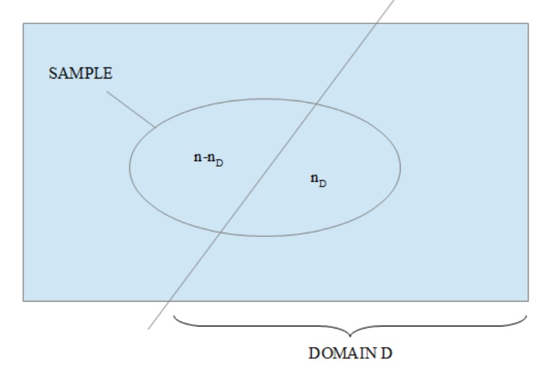
Figure 2.1: Domain estimation

When the size \(N_D\) of \(U_D\) is known, we can use the following formula as an alternative to \(\hat{Y}_D\): \[\begin{equation} \hat{Y}_{D,alt} = N_D \bar{y}_D \tag{2.16} \end{equation}\]

Using the main results for simple random sampling, we obtain the following:

• Result 1: Assuming the population sizes \(N\) and \(N_D\) are large enough, the variance of the domain estimator \(\hat{Y}_D\) is given by: \[\begin{equation} V\left(\hat{Y}_D\right) \approx N^2_D \left(1/\bar{n}_D-1/N_D\right)S_D^2\left(1 + \frac{1-P_D}{CV^2_D}\right) \tag{2.17} \end{equation}\]

where:

\(S_D^2 = \sum_{k \in U_D} \left(y_k - \bar{Y}_D\right)^2 / \left(N_D-1\right)\)

\(CV_D = S_D / \bar{Y}_D\)

• Result 2: Assuming the sample size \(n_D\) is large enough, the variance of \(\hat{Y}_{D,alt}\) is given by: \[\begin{equation} V\left(\hat{Y}_{D,alt}\right) \approx N^2_D \left(1/\bar{n}_D-1/N_D\right)S_D^2 \tag{2.18} \end{equation}\]

• Result 3: The variance of \(\hat{Y}_{D,alt}\) is lower than that of \(\hat{Y}_{D}\): \[\begin{equation} \begin{array}{lcl} V\left(\hat{Y}_{D,alt}\right) / V\left(\hat{Y}_D\right) & \approx & 1 / \left(1 + {\displaystyle \frac{1-P_D}{CV^2_D}}\right) \\ & = & CV^2_D / \left(CV^2_D + Q_D\right) \end{array} \tag{2.19} \end{equation}\]