Survey data in the field of economy and finance
2021-11-07
Chapter 1 Introduction
1.1 History
Counting a population through censuses has been a long established practice which dates back to thousand years BC. Babylonians, Egyptians, Romans etc. used to resort to population censuses to support important economic decisions in terms of taxation, labour force scaling, food distribution etc. Censuses are usually regarded as error-free data sources leading to statistics with highest accuracy. On the other hand, censuses are also long and expensive operations which take very long time (often several years) in order to be fully prepared and implemented. Thus, they cannot be conducted on a frequent basis. Nowadays, many European countries, including Luxembourg, carry out population censuses every ten years.
In order to produce updated statistical figures between two census periods, sample surveys have proven to be powerful instruments, although it took very long for the scientific community to validate the idea that collecting data over a sample of a population may lead to as accurate results as for a census. Actually, the rise of survey sampling in modern statistical production started recently in the second half of the 20th century when it was shown that probability theory, especially the Central Limit Theorem, could be used to compute valid confidence intervals and margins of errors for survey estimates based on probability samples. This has given rise to a full body of sampling theory, where Probability and Mathematics are mobilized with the aim of improving sampling efficiency and making data accuracy better.
Nowadays sample surveys are commonly used by data producers (National statistics institutes, central banks, public administrations, universities, research centres, private businesses etc.) as a key source of statistical information on a wide variety of domains such as economy, finance, demography, sociology, environmental research, biology or epidemiology.
1.2 Examples of surveys
In Luxembourg, the National Statistical Institute (STATEC)1 regularly conducts a lot of sample surveys targeting the households, individuals and businesses in the country.
> Example 1: List of all the household surveys conducted by Luxembourg’s STATEC
- Social life
- Household Budget Survey
- Safety Survey
- Time Use Survey
- Business and Leisure Tourism Survey
- European Statistics on Income and Living Conditions
- Community Survey on the Usage of Information and Communications Technologies (ICT) among Households and Individuals
- Labour market and education
- Labour Force Survey
- Adult Education Survey
- Population and housing
- Population and Housing Census
- Statistics of Completed Buildings Survey
- Statistics of Transformation Survey
- Price
- Rents Survey
- Housing Characteristics Survey
- Quality
- Confidence in Public Statistics
Central banks are also increasingly resorting to survey data as an addition to macro-economic aggregates in order to help them monitor financial stability, assess tail risks or study new policy needs.
> Example 2: List of the surveys supervised by the European Central Bank
- Survey of monetary analysts (SMA)
- ECB survey of professional forecasters (SPF)
- Bank lending survey (BLS)
- Survey on the access to finance of enterprises (SAFE)
- Household finance and consumption survey (HFCS)
- Survey on credit terms and conditions in euro-denominated securities financing and over-the-counter derivatives markets (SESFOD)
- Consumer expectations survey (CES)
Quoting ECB’s website2: "These surveys provide important insights into various issues, such as:
- micro-level information on euro area households’ assets and liabilities
- financing conditions faced by small and medium-sized enterprises
- lending policies of euro area banks
- market participants’ expectations of the future course of monetary policy
- expectations about inflation rates and other macroeconomic variables
- trends in the credit terms offered by firms in the securities financing and over-the-counter (OTC) derivatives markets, and insights into the main drivers of these trends."
A great deal of international survey programs have also been developed by academic consortiums to address important research questions. Those studies provide comparable micro-data between the participating countries. Among many examples, we can mention the European Social Survey (ESS)3, the European Values Study (EVS)4, the Survey On Health Ageing and Retirement in Europe (SHARE)5, the International Crime and Victim Survey (ICVS)6 or the Global Monitor Entrepeneurship (GEM)7
1.3 Pros and cons of surveys
Compared to exhaustive enumerations, sample surveys provide results much faster and at reduced cost. This makes surveys highly relevant when statistics are quickly needed and the resources available (in terms of staff, time and money) are limited.
Furthermore, surveys can focus on topics censuses cannot deal with in too much detail, for example:
- For households and individuals: household income, consumption, wealth or indebtedness, time use, victimization experiences, internet usage, tourism activities, financial difficulties, material deprivation, personal health, education and training, work-life balance or any subjective aspects (opinions, attitudes, values, perceptions etc.);
- For businesses: R&D investment, business turnover, credit conditions, agricultural production, financial risk or market expectations.
Surveys also collect a great deal of control variables which can be used for statistical modeling. For example, the European Statistics on Income and Living Conditions (EU-SILC)8 consist of a set of sample surveys which are conducted in every European countries over representative samples of thousands of households and individuals. They collect a great deal of key socio-economic covariates at individual and household level on age, gender, citizenship, education, health, family status, living arrangements, dwelling conditions, housing burden, financial difficulties etc. in addition to the target income variables. All this information can be used to build sophisticated income models and identify income drivers.
Another strong advantage of sample surveys is they provide unit-level data that is, micro-data. Thus, comparisons are possible between sub-populations of interest (e.g. based on age, gender, citizenship, income groups, geographical region, company size etc.), which makes the survey instrument highly suited for studying distributional aspects and inequalities. For example, the EU-SILC database has become the reference source of micro-data for the European countries, producing key indicators on income poverty and inequality, such as poverty rates, quantile ratios or concentration measures such as the Gini coefficient. As to ECB’s Household Finance and Consumption Survey (HFCS)9, it collects detailed micro-data on household wealth and indebtedness. The HFCS is a key source to analyze wealth inequality between households and help monitor financial stability through developing debt sustainability models based on household idiosyncratic shocks.
On the other side, surveys suffer from a very specific kind of errors, called sampling errors, caused by collecting partial information over a fraction of the population rather than the whole population itself. As a result, survey data cannot produce exact values but only estimates of population quantities, whose accuracy depends on the sample size: the higher the size the better the accuracy. Therefore, sample size is an important limitation to the design and implementation of surveys. Furthermore, surveys, like censuses, also suffer from non-sampling errors caused by factors other than sampling (e.g measurement, coverage or non-response errors).
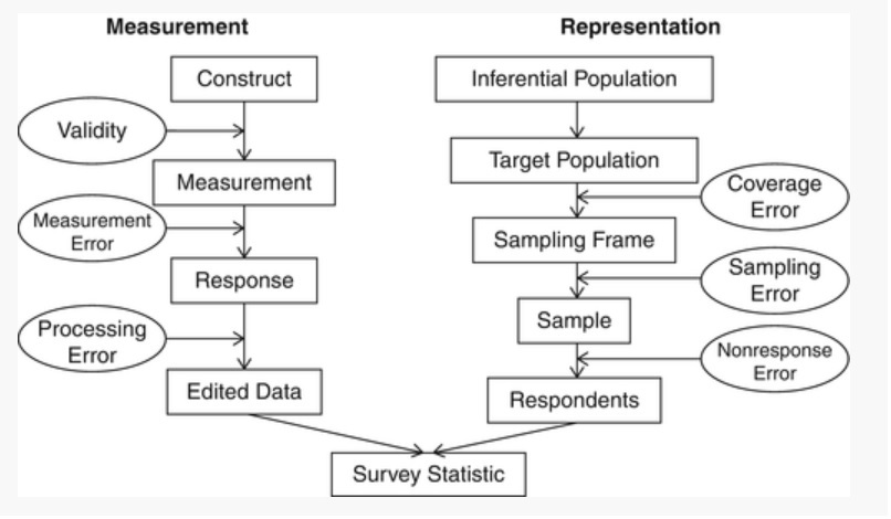
Figure 1.1: Sources of survey errors (Groves et al., 2004)
However, provided they are designed and conducted properly, sample surveys may in fact happen to be (at least) as efficient as censuses as the magnitude of non-sampling errors is generally smaller when data are collected over a sample of population units than they are in case of a census.
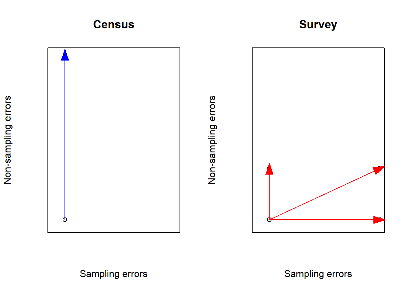
That’s why, in order to outperform censuses, it is key that sample surveys be designed and conducted in a way to make non-sampling errors the smallest possible. Concretely, significant resources must be devoted to keep sampling errors under control; survey questionnaires must be prepared with utmost care, intensively pre-tested and field-tested in order to detect issues in question wording, routing problems or any other inconsistency; the modes of data collection must be chosen and combined judiciously in order to get most people to cooperate; the interviewers must be carefully recruited and properly trained; communication and contact strategies towards participants must be designed and adapted in order to reach highest participation.
1.4 Main concepts and definitions
1.4.1 Population, sample; parameter and estimator
\(U\) denotes a finite population of \(N\) units. Statistical units must be regarded as a broad concept: physical individuals, households, dwellings, businesses, agricultural farms, animals, cars, manufactured objects etc. can be considered as units for statistical purposes. It is assumed that every unit \(i \in U\) can be fully and unambiguously identified through a label. For instance, a physical person can be identified through its name, surname, gender, date of birth and postal address. A business could be identified using its VAT number or its registration number in a business register.
We wish to estimate a population parameter \(\theta\), defined as a function of the \(N\) values taken by a study variable \(\mathbf{y}\) over each element of the population \(U\):
\[\begin{equation} \theta = \theta\left(\mathbf{y}_i , i \in U\right) \tag{1.1} \end{equation}\]
\(\mathbf{y}_i\) can be either a quantitative (e.g. the total disposable income or the total food consumption of \(i\)) or a categorical information (e.g. gender, citizenship, country of birth, marital status, occupation or activity status). In the followibg, \(y\) is supposed to be observed without any error.
\(\theta\) can be a linear parameter of \(\mathbf{y}\), such as a mean, a total or a proportion, or a more complex one such as a ratio between two population means, a correlation or a regression coefficient, a quantile (e.g. median, quartile, quintile or decile) or an inequality measure such as the Gini or the Theil coefficient.
In a survey setting, a sample \(s\) of \(n\) units \(\left(n \leq N\right)\) is taken from \(U\). When a sample is selected according to a probabilistic design, then every element in the population has a fixed known in advance probability to be selected: the probability \(\pi_i\) for a unit \(i \in U\) to be sampled is called the inclusion probability. Otherwise, when the inclusion probabilities are unknown, then the design is said to be empirical. This is what happens for instance in quota sampling, whereby units are selected so to reflect known structures for the population, in expert sampling, whereby sample units are designated from expert advice or in network sampling, whereby the existing sample units recruit future units from among their ‘network’.
In the following, it is assumed sample units are selected through a probabilistic design. In which case, the sample \(s\) can be regarded as the realization of a random variable \(S\). In most cases, \(s\) is a subset without repetitions of the population (sampling without replacement), although a sample can also be taken with replacement. Sample observations are used to construct an estimator of the parameter \(\theta\), that is a function of sample observations:
\[\begin{equation} \hat\theta = \hat\theta\left(S\right) = \hat\theta\left(\mathbf{y}_i , i \in S\right) \tag{1.2} \end{equation}\]
For instance, the population mean of the study variable can be estimated by the mean value over the sample observations (see next chapter):
\[\begin{equation} \hat\theta = \frac{\sum_{i \in S} \mathbf{y}_i}{\#S} = \bar{\mathbf{y}}_S \tag{1.3} \end{equation}\]
The size of the selected sample is another example of estimator:
\[\begin{equation} n_S = \sum_{i \in S} 1 \tag{1.4} \end{equation}\]
When \(n_S = n\) then the design is of fixed size.
In survey sampling theory, as the study variable is assumed to be error-free, the random part of an estimator is caused by the probabilistic selection of a sample. This is a major difference in comparison to traditional statistical theory, where the study variable is assumed to follow a given probability distribution (e.g. a normal distribution of mean \(m\) and standard error \(\sigma\))
1.4.2 Sampling frame
The selection of a sample in a population requires a sampling frame that is, an exhaustive list of all the individuals which comprise the target population. For example, Luxembourg has a Population Register in which the whole resident population is supposed to be recorded. This register is used by STATEC to draw samples for its household surveys. Similarly, there exists in Luxembourg a Business Register which is used as a basis to business surveys.
In practice, frames are not error-free: while they can never encompass the whole target population (because it always takes time to administrativally record an individual in a register), they also contain individuals which are no longer eligible (e.g. individuals who left the country and may keep recorded in the Register several months after they left). Discrepancies between the (theoretical) target population of a survey and the frame which is used to draw a sample are equivalent to statistical errors, called coverage errors or frame errors.
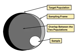
Figure 1.2: Coverage errors
1.4.3 Bias, Variance, Standard error and Mean Square Error
Under probabilistic sampling, several synthetic measures are available in order to assess the statistical quality of an estimator \(\hat\theta\). All these measures are equivalent to those developed in classical statistics theory:
- Expectation
This is the average value of \(\hat\theta\) over all the possible samples \(\mathcal{S}\) that can be taken from the population:
\[\begin{equation} E\left(\hat\theta\right) = \sum_{s \in \mathcal{S}}Pr\left(S=s\right)\hat\theta\left(S=s\right) \tag{1.5} \end{equation}\]
- Bias
The bias of the estimator \(\hat\theta\) is given by:
\[\begin{equation} B\left(\hat\theta\right) = E\left(\hat\theta\right) - \theta \tag{1.6} \end{equation}\]
If \(B\left(\hat\theta\right)=0\), the estimator \(\hat\theta\) is said to be unbiased. Bias is not measurable as the true value \(\theta\) of the parameter is unknown.
- Variance
The variance of the estimator \(\hat\theta\) is given by:
\[\begin{equation} V\left(\hat\theta\right) = E\left[\hat\theta - E\left(\hat\theta\right)\right]^2 = E\left(\hat\theta^2\right) - E^2\left(\hat\theta\right) \tag{1.7} \end{equation}\]
By taking the square root of the variance, we obtain the standard error:
\[\begin{equation} \sigma\left(\hat\theta\right) = \sqrt{V\left(\hat\theta\right)} \tag{1.8} \end{equation}\]
When the standard error is expressed as a percentage of the parameter \(\theta\), we got the relative standard error or coefficient of variation:
\[\begin{equation} CV\left(\hat\theta\right) = \frac{\sqrt{V\left(\hat\theta\right)}}{\theta} \tag{1.9} \end{equation}\]
- Mean Square Error
The mean square error is a synthetic quality measure summarising bias and variance:
\[\begin{equation} MSE\left(\hat\theta\right) = E\left(\hat\theta - \theta\right)^2 = V\left(\hat\theta\right) + B^2\left(\hat\theta\right) \tag{1.10} \end{equation}\]
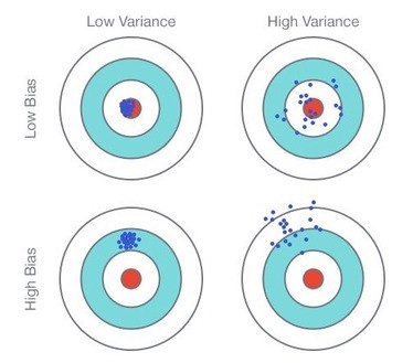
Figure 1.3: Comparison Bias/Variance
We’ll see that the quality of a statistical estimator is often regarded as a tradeoff between bias and variance. In general, bias is often regarded as a major problem and we seek to keep its level as low as possible. Variance is also a problem but we’ll see it is directly related to sample size: therefore the bigger the sample, the lower the variance. On the contrary, bias is harder to deal with as it is related to other factors such as the survey questionnaire or the mode of data collection.
Numerical example: Consider a population of \(N\)=10 elements, labelled \(i = 1 \cdots 10\), and a study variable \(y_i\) for every population elements. \[\begin{array}{|c|c|} i & \textbf{y} \\ 1 & 2 \\ 2 & 5 \\ 3 & 8 \\ 4 & 4 \\ 5 & 1 \\ \end{array}\]Consider a sampling design in which every sample of size 2 has the same probability, equal to 1/10, to be selected. The probability is zero when the size of the sample is not equal to 2.
We seek to estimate the population mean of the study variable \(y\) that is, \(\bar{Y} = \displaystyle{\frac{y_1 + y_2 + y_3 + y_4 + y_5}{5}} = 4\). To that end, we use the sample mean \(\bar{y}\) as an estimator of \(\bar{Y}\).
We got the following: \[\begin{array}{|c|c|c|} s & Pr\left(S=s\right) & \bar{y} \\ \{1,2\} & 0.1 & 3.5 \\ \{1,3\} & 0.1 & 5.0 \\ \{1,4\} & 0.1 & 3.0 \\ \{1,5\} & 0.1 & 1.5 \\ \{2,3\} & 0.1 & 6.5 \\ \{2,4\} & 0.1 & 4.5 \\ \{2,5\} & 0.1 & 3.0 \\ \{3,4\} & 0.1 & 6.0 \\ \{3,5\} & 0.1 & 4.5 \\ \{4,5\} & 0.1 & 2.5 \\ \end{array}\]The bias of the sample mean is given by: \(0.1 \left(3.5 + 5.0 + 3.0 + 1.5 + 6.5 + 4.5 + 3.0 + 6.0 + 4.5 + 2.5\right) = 4 = \bar{Y}\)
Therefore the estimator is unbiased. As regards the variance, we have: \[\begin{array}{|c|c|c|} s & Pr\left(S=s\right) & \left(\bar{y}-\bar{Y}\right)^2 \\ \{1,2\} & 0.1 & 0.5^2 \\ \{1,3\} & 0.1 & 1.0^2 \\ \{1,4\} & 0.1 & 1.0^2 \\ \{1,5\} & 0.1 & 2.5^2 \\ \{2,3\} & 0.1 & 2.5^2 \\ \{2,4\} & 0.1 & 0.5^2 \\ \{2,5\} & 0.1 & 1.0^2 \\ \{3,4\} & 0.1 & 2.0^2 \\ \{3,5\} & 0.1 & 0.5^2 \\ \{4,5\} & 0.1 & 1.5^2 \\ \end{array}\]The variance of the sample mean is given by: \(0.1 \left(0.25 + 1.0 + 1.0 + 6.25 + 6.25 + 0.25 + 1.0 + 4.0 + 0.25 + 2.25\right) = 2.25\)
1.4.4 Confidence interval
Ultimately, the estimated standard error is used to determine a confidence interval in which the target parameter \(\theta\) lies with very high probability, which is close to 1. The statistical process extrapolating results from sample observations to the whole population (in the form of a confidence interval) is called statistical inference.
Assuming the estimator \(\hat\theta\) is unbiased and normally distributed, a confidence interval for \(\theta\) at level \(1 - \alpha\) is given by:
\[\begin{equation} CI\left(\theta\right) = \left[\hat\theta - q_{1-\alpha/2}\times \sigma\left(\hat\theta\right) ~,~ \hat\theta + q_{1-\alpha/2}\times\sigma\left(\hat\theta\right)\right] \tag{1.11} \end{equation}\]
where \(q_{1-\alpha/2}\) is the quantile at \(1-\alpha/2\) of the normal distribution of mean 0 and standard error 1. For instance, we have:
- \(\alpha = 0.1 \Rightarrow q_{1-\alpha/2}=1.65\)
- \(\alpha = 0.05 \Rightarrow q_{1-\alpha/2}=1.96\)
- \(\alpha = 0.01 \Rightarrow q_{1-\alpha/2}=2.58\)
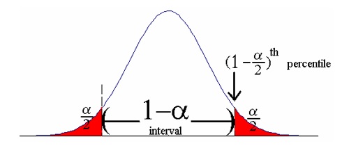
Figure 1.4: Confidence interval
The quantity \(q_{1-\alpha/2} \times \sigma\left(\hat\theta\right)\) that is, the half-length of the confidence interval, is the (absolute) margin of error. When the latter is expressed as a percentage of \(\theta\), we got the relative margin of error.
In practice the standard error \(\sigma\left(\hat\theta\right)\) is unknown and therefore is estimated by \(\hat\sigma\left(\hat\theta\right)\). Thus, we obtain the following estimated confidence interval through substituting \(\hat\sigma\left(\hat\theta\right)\) for \(\sigma\left(\hat\theta\right)\):
\[\begin{equation} \hat{CI}\left(\theta\right) = \left[\hat\theta - q_{1-\alpha/2}\times \hat\sigma\left(\hat\theta\right) ~,~ \hat\theta + q_{1-\alpha/2}\times \hat\sigma\left(\hat\theta\right)\right] \tag{1.12} \end{equation}\]
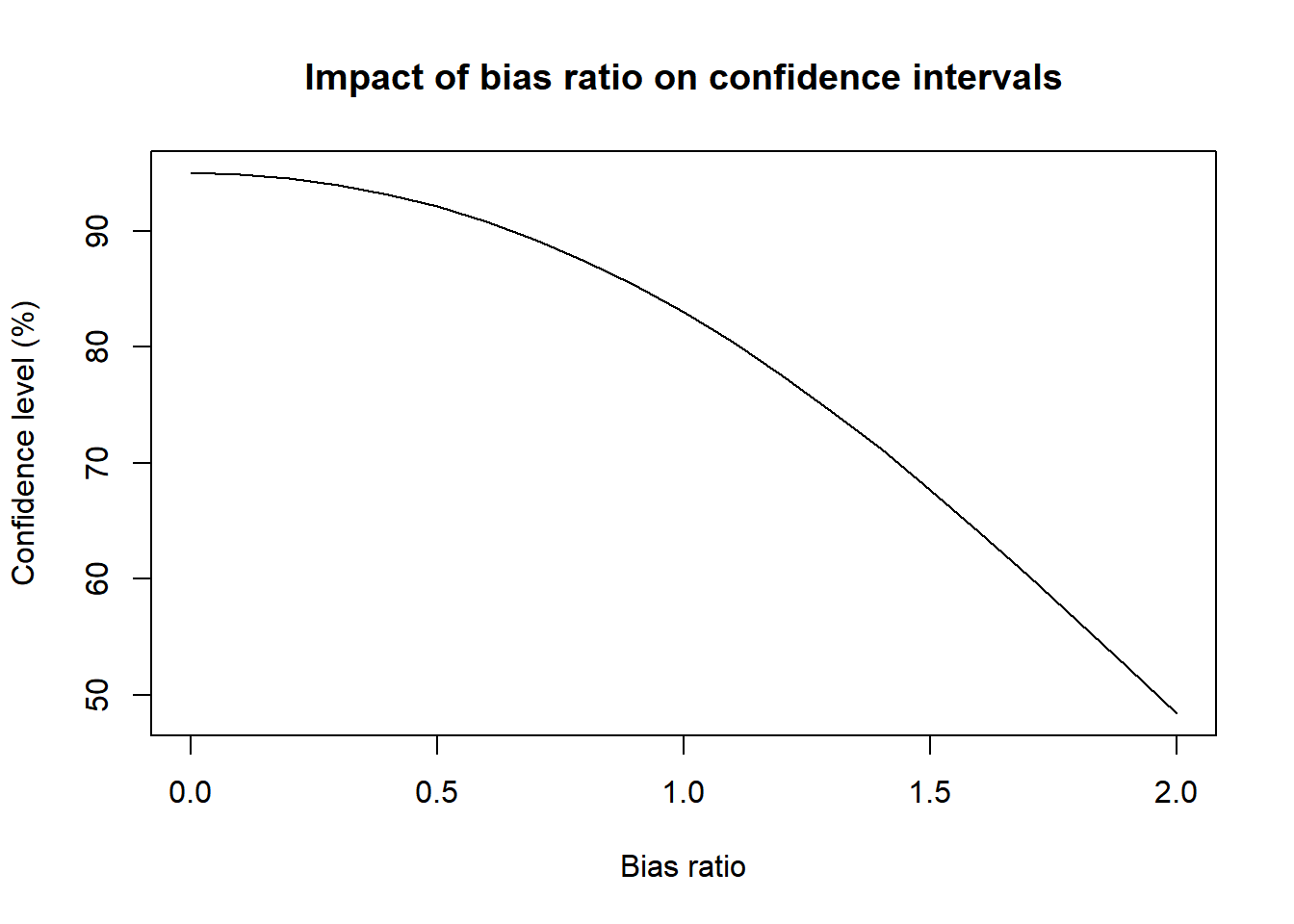
The normality assumption which underlies (1.11) generally holds provided the sample size is large enough. When the sample size is too small, the quantile \(q_{1-\alpha/2}\) can be replaced by the quantile of the t-distribution (Student) with degrees of freedom \(n-1\). As regards unbiasedness, this property can be verified under ideal conditions (e.g. simple random sampling). However, it is not satisfied under general survey conditions, mainly because of the negative effect of non-sampling errors. In this case, bias leads to distorting the confidence level in the sense the theoretical value \(1 - \alpha\) is actually higher than the real value when the bias ratio \(B\left(\hat\theta\right) / \sigma\left(\hat\theta\right)\) is too high:
Confidence intervals are easy to understand and interpret, contrary to the more complex indicators of variance and standard error. The two latter are in fact not the ultimate goal in statistical inference, but rather an intermediary step towards the construction of confidence intervals.