2 Information Processing with R
2.1 Getting R and R Studio
Before we start with the basics of R make sure you have the latest version of R. To install R as a desktop app, go to the R Project website. For development, an Integrated Development Environment (IDE) is recommended. R Studio is the leading IDE for R and can be obtained from . Rather than installing R and R Studio on your desktop, you can also use a cloud version at RStudio.cloud.
2.1.1 32-bit vs 64-bit R
On Windows you have achoice between a 32-bit and a 64-bit version of R. We recommend you use the 64-bit version and that you allow R to auto-detect the rendering engine. The 64-bit version allows for larger objects and allows your program to use more than 2GB of memory (32-bit addressing limits you to a max of 4GB but Windows reserves 2GB for the operating systems). The 32-bit version of R is provided for backwards compatibility with older packages and is only used when a package does not have a 64-bit version. Using the cloud version eliminates those choices.
2.2 Basic R
Data is generally stored in R as a dataframe. A dataframe is similar to a spreadsheet in that is has columns and rows. Each row holds a data record (also called an observation, a case, a row, or an object). All values in a column must be of the same type. Dataframes are created by:
- Reading data from an external file
- Retrieving data from a URL
- Creating an object directly from the command line
- Instantiating an object from within a program
2.2.0.1 Expressions
R can be directly used to solve simple or complex mathematical expressions.
12*21## [1] 252# [1] in the above answer indicates the index of your results.
# R always shows the result with index for each row.
((2^3)*5)-1## [1] 39# sqrt and exp are built-in functions in R for finding Square root and exponential respectively.
sqrt(4)* exp(2)## [1] 14.778112.2.0.2 Variables & Identifiers
Holding a value in a variable is done through assignment. Once you assign a value to a variable, the variables becomes an R object. There are two ways to do an assignment, with a ‘=’ and with a ‘<-’. The latter is the preferred way in R.
Note that variables do not need to be explicitly defined. The first time a variable is assigned a value defines the variable and its type. The type is based on the value that is assigned. Unlike other programming languages such as C++, C#, or Java, R is not strongly typed: the type of a variable can change when a value of a different type is assigned. A variable can be used in an expression. Its value can be inspected by just using the variable by itself.
The value of a variable can be displayed either by using the variable by itself or using the print() function.
# assignment with '=' of a number
x = 12
# inspect (print/display) the value
x
## [1] 12# assignment a new value and change its type to "text"
x = "Hello"
x## [1] "Hello"# assignment with '<-'
x <- 12
print(x)## [1] 12The rules for naming an identifier (variable, function, or package name) for an object are as follows:
- identifiers are case-sensitive and cannot contain spaces or special characters such as #, %, $, @, *, &, ^, !, ~
- an identifier must start with a letter, but may contain any combination of letters and digits thereafter
- special characters dot (.) and underscore (_) are allowed
The dot (.) is a regular character in R and that can be confusing as other language (e.g., Java) use dot to designate property or method access, e.g, in Java x.val means that you are accessing the val property of the object x.
Some examples of legal variable names are: df, df2, df.txns, df_all2017. These are some illegal variable names: 2df (cannot start with a digit), rs$all (cannot contain a $; the $ is used to access columns in a dataframe), rs# (only . and _ are allowed in addition to digits and letters).
It is considered good programming practice to give identifiers a sensible name that hints as to what is stored in the variable rather than using random name like x, val, or i33. Identifiers should be named consistently. Many programmers use one of two styles:
- underscores, e.g., interest_rate
- camelCase, e.g., squareRoot, graphData, currentWorkingDirectory
Note that R is case sensitive which means that R treats the identifiers AP and ap as different objects. As a side note, files may also be case sensitive but that depends on the operating system. MacOS and Linux are case sensitive, while Windows is case aware but not case sensitive. For example, on MacOS and Linux there is a difference between “AirPassengers.txt” and “airpassengers.txt” while on Windows there is not. SQL is also not case sensitive. It is a best practice to assume case sensitivity.
2.2.0.3 Coercion
Types can be converted using as.xxxx functions, e.g., as.numeric(), as.date() or as.string(). Conversions are often necessary when data is read from CSV or XML files or databases as the data is always text (strings).
x <- 3.14
v <- as.integer(x)    # removes fraction (no rounding)

s <- "3.14"           # numbers in quotes are text: s + 1 would be an error
w <- as.numeric(s)    # converts text to a number
w <- w + 2.71
2.2.0.4 Rounding
x <- 23 / 77
print(x)
## [1] 0.2987013w <- round(x,3) # round to three decimals
print(w)## [1] 0.299w <- floor(x) # round down to nearest integer
print(w)## [1] 0w <- ceiling(x) # round up
print(w)## [1] 1w <- trunc(x) # remove decimals
print(w)## [1] 02.2.1 Functions
R has numerous built-in functions. Many more are found in the hundreds of packages (libraries of functions) available for download. R functions are invoked (or called) by using their name with parenthesis after. The parenthesis distinguish a function from a data object.
2.2.1.1 Function Documentation
Details of any built-in functions can be accessed by adding a question mark (?) in front of the function. More information can generally be found through a web search.
?sumNote that in R the arguments do not have to be passed in the order in which the functions expects them as long as you state which argument you are passing.
2.2.2 Built-in Datasets
R has numerous built-in datasets that are useful for testing and learning R. They should not be used for any actual analysis. Some examples are mtcars, sunspots. Most built-in datasets are dataframe objects. Using the head() and tail() functions is recommended so that only the first few or the last few rows of a dataframe are displayed when inspecting a dataframe.
mtcars # displays the full data framehead(mtcars) # displays only first 6 rows## mpg cyl disp hp drat wt qsec vs am gear carb
## Mazda RX4 21.0 6 160 110 3.90 2.620 16.46 0 1 4 4
## Mazda RX4 Wag 21.0 6 160 110 3.90 2.875 17.02 0 1 4 4
## Datsun 710 22.8 4 108 93 3.85 2.320 18.61 1 1 4 1
## Hornet 4 Drive 21.4 6 258 110 3.08 3.215 19.44 1 0 3 1
## Hornet Sportabout 18.7 8 360 175 3.15 3.440 17.02 0 0 3 2
## Valiant 18.1 6 225 105 2.76 3.460 20.22 1 0 3 1head(mtcars,2) # displays only first 2 rows## mpg cyl disp hp drat wt qsec vs am gear carb
## Mazda RX4 21 6 160 110 3.9 2.620 16.46 0 1 4 4
## Mazda RX4 Wag 21 6 160 110 3.9 2.875 17.02 0 1 4 42.2.3 Vectors
Vectors, a collection of numbers or text, are another fundamental object type in R. Vectors can be generated as sequences or collections.
v <- c(2,9,3,11)          # vector of four numbers
sum(v)                    # add the numbers in the vector
## [1] 25v <- 10:30 # vectors of numbers from 10 to 30
v <- seq(10,100,by = 5) # vector of multiples of 5
# vector of text (string) objects
v <- c("Northeastern","MIT","Cornell")
l <- length(v) # length (number elements)
# vector og logical (boolean) values
logical.vec<- c(T,F,F,T,F,T,T)
logical.vec## [1] TRUE FALSE FALSE TRUE FALSE TRUE TRUEVectors can be concatenated, i.e., put together.
v <- c(1,3,5,7,11)
w <- c(1,2,3,5,8)

q <- c(v,w)
q
## [1] 1 3 5 7 11 1 2 3 5 8q <- round(q,2) # round all valuesVectors of the same length can also be used in algebraic operators, such as addition, subtraction, etc. For example, adding two vectors adds each of the elements in the same position, i.e., \(v=\{v_1,v_2,...,v_n\}\) + \(w=\{w_1,w_2,...,w_n\}\) results in \(\{v_1+w_1,v_2+w_2,...,v_n+w_n\}\). Vectors of unequal length only add the number of elements of the smallest vector.
v <- c(1,3,5,7,11)
w <- c(1,2,3,5,8,13)
v + w
## Warning in v + w: longer object length is not a multiple of shorter object
## length## [1] 2 5 8 12 19 14r <- v / w## Warning in v/w: longer object length is not a multiple of shorter object
## length2.2.4 Factors
The Factor data type type is used to encode categorical data values. While a vector can have any number of distinct elements, a factor value is limited to its categories. Factors are essential for certain statistical hypothesis tests and models. Factors are stored as numbers internally but no algebraic operations such as subtraction are defined for factors.
In section 2.9.1, we will learn that when text files, including CSV, are read into a dataframe then all text is converted to factors unless that conversion is suppressed.
Factors can also be explicity created using the factor() function which requires a vector of category values as input.
# create a factor variable from a vector of strings
week <- c("Monday","Tuesday","Wednesday","Thursday","Friday","Saturday","Sunday")
fac <- factor(week)
print(fac)
## [1] Monday Tuesday Wednesday Thursday Friday Saturday Sunday
## Levels: Friday Monday Saturday Sunday Thursday Tuesday WednesdayWhen you create a factor from a data object you can provide a default ordering for the values. If you do not provide an ordering it will use the canonical ordering for the data type so ascending order for numeric data and alphabetical ordering for character data. Since you probably do not want to order the days of the week alphabetically, here is an example of specifying the ordering sequence with the factor function
week = c("Monday","Tuesday","Wednesday","Thursday","Friday","Saturday","Sunday")
fac.ordered <- factor(week, labels=week, ordered=TRUE)
print(fac.ordered)
## [1] Tuesday Saturday Sunday Friday Monday Wednesday Thursday
## 7 Levels: Monday < Tuesday < Wednesday < Thursday < ... < SundayFactors have labels and levels. The level is numeric and provides an ordering but they should not be considered numbers. In fact, R treats them as the factor data type rather than numeric. Mathematical operations are not defined.
labels(fac)## [1] "1" "2" "3" "4" "5" "6" "7"levels(fac)## [1] "Friday" "Monday" "Saturday" "Sunday" "Thursday" "Tuesday"
## [7] "Wednesday"labels(fac.ordered)## [1] "1" "2" "3" "4" "5" "6" "7"levels(fac.ordered)## [1] "Monday" "Tuesday" "Wednesday" "Thursday" "Friday" "Saturday"
## [7] "Sunday"Using factor variables as numeric results in an error.
mean(fac)## Warning in mean.default(fac): argument is not numeric or logical: returning
## NA## [1] NAFactor variables can be re-configured and new levels can be added and removed.
week <- c("Monday","Tuesday","Wednesday","Thursday","Friday","Saturday","Sunday")
fac <- factor(week)

workweek <- week[week != "Sunday"]
workweek <- week[week != "Saturday"]
fac.workdays <- factor(workweek, labels=workweek, ordered=TRUE)
print(fac.workdays)
## [1] Tuesday Friday Sunday Thursday Monday Wednesday
## Levels: Monday < Tuesday < Wednesday < Thursday < Friday < Sunday2.2.5 Matrices
A matrix is a two-dimensional arrangement of data similar to a data frame but unlike a data frame its elements must be of the same data type. To perform mathematical operations on matrices, its elements must be numeric. When a matrix is printed the output contains the name of the columns in the first row. Each row element is prefixed with a row number.
mat<- matrix(c(1:10), nrow=5, ncol=4, byrow= TRUE)
print(mat)
## [,1] [,2] [,3] [,4]
## [1,] 1 2 3 4
## [2,] 5 6 7 8
## [3,] 9 10 1 2
## [4,] 3 4 5 6
## [5,] 7 8 9 102.2.5.1 Matrix Operations
R supports many common matrix operations. The function t() creates a transpose of a matrix by interchanging its columns and rows.
t(mat)## [,1] [,2] [,3] [,4] [,5]
## [1,] 1 5 9 3 7
## [2,] 2 6 10 4 8
## [3,] 3 7 1 5 9
## [4,] 4 8 2 6 102.3 Common Statistical Functions
2.3.0.1 Random Numbers and Samples
# vector of 4 random numbers
runif(4)
## [1] 0.6742811 0.5015733 0.5387205 0.6531705# vector of 3 random numbers from 0 to 100
runif(3, min=0, max=100)## [1] 6.00070 91.23219 13.93401# vector of 3 random integers from 0 to 100
# use max=101 because it will never actually equal 101
floor(runif(3, min=0, max=101))## [1] 56 43 25# same result but using a different approach
sample(1:100, 3, replace=TRUE)## [1] 95 37 3# random sample WITHOUT replacement:
sample(1:100, 3, replace=FALSE)## [1] 4 27 76# sample of random numbers from normal distribution
rnorm(4)## [1] 0.9344520 0.4938148 -0.6798735 -2.0445359# use different mean and standard deviation parameters
rnorm(10, mean=50, sd=10)## [1] 42.95891 45.76986 53.41746 70.54035 38.67652 39.28500 56.67896
## [8] 54.27074 55.72783 56.037932.3.1 Histograms
Histograms (or frequency plots) are commonly used to visually inspect the distribution of a set of numbers.
# visualize distribution using a histogram of the numbers
x <- rnorm(500, mean=50, sd=10)

hist(x)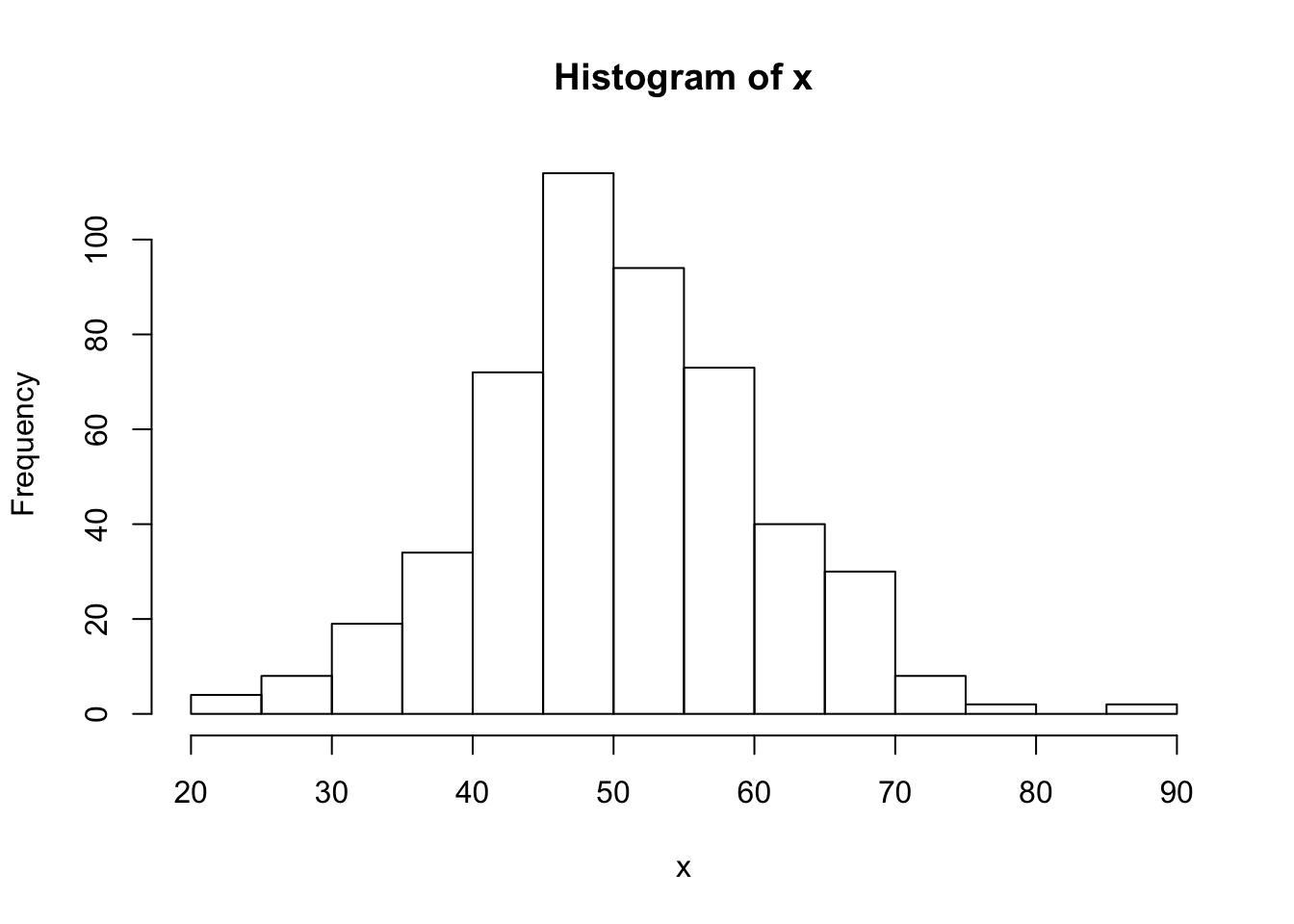
2.3.2 Simple Desriptive Statistics
# create a vector of 100 random numbers
v <- runif(100, min=0, max=1000)

mean(v)              # mean (average)
## [1] 525.0826mean(v, trim=0.1) # 10% trimmed mean## [1] 529.5522median(v) # median (middle in ordered list)## [1] 550.8823sd(v) # standard deviation## [1] 279.8727var(v) # variance (sd squared)## [1] 78328.74range(v) # min and max values## [1] 2.923421 992.765642IQR(v) # interquartile range## [1] 390.96292.3.3 Missing Values
Missing values are indicated in R with the NA object. Many functions can automatically ignore or remove missing values.
# create a vector
x <- c(11,7,3,4.7,18,2,NA,54,-31,8,-6.2,NA)

x.mean <-  mean(x)
print(x.mean)
## [1] NA# mean with NA dropped
x.noNA.mean <- mean(x,na.rm = TRUE)
print(x.noNA.mean)## [1] 7.052.4 Flow Control
Often code needs to be executed conditionally or repeatedly. For such situations, R, like most programming languages, offers flow control statements, including if, switch, and for.
2.4.1 Conditional Execution: if
An if statement allows for conditional execution of one or more statements. Whether the code is run depends on whether the boolean_expression evaluates to \(TRUE\).
if (boolean_expression) {
   # statement(s) will execute if the boolean expression is true.
}
2.4.1.1 Boolean Expressions
The boolean_expression consists of one or more logical statements. Multiple statements are connected with logical operators AND (&), OR (|) and NOT (!). The logical operators are summarized in the table below.
| Operator | Description |
|---|---|
| < | less than |
| <= | less than or equal to |
| > | greater than |
| >= | greater than or equal to |
| == | exactly equal to |
| != | not equal to |
| !x | not x |
| x | y |
| x & y | x AND y |
| isTRUE(x) | test if X is TRUE |
In boolean algebra, \(\land\) means AND \(\lor\) means OR, and \(\neg\) means NOT. AND is only \(true\) if both operands are true. OR is true if either or both operands are \(true\).
2.4.1.2 DeMorgan’s Laws
DeMorgan’s Laws can be used to simplify certain boolean expressions.
\(\neg (p\land q) \longleftrightarrow (\neg p \lor \neg q)\)
\(\neg (p\lor q) \longleftrightarrow (\neg p \land \neg q)\)
together with double negation elimitation
\(\neg \neg p \longleftrightarrow p\)
may be used to convert between conjuctive and disjunctive boolean expressions, but notice you’ll often need negation too.
2.4.2 Iteration and Loops
There are times when some block of code needs to execute several number of times, perhaps once for each element of a vestor or each row in a file. Most programming languages provide various control structures that allow for looping where a statement is executed several times or until some condition is met.
R offers three different loop statements: for, repeat, and while.
2.4.2.1 for Loop
A for is most commonly used to execute some block of statements for some number of times.
# add up all the numbers in a sequence
s <- 0
for (i in 1:5)
{
  s <- s + i
  print(paste("i = ", i, " | s = ", s))
}
## [1] "i = 1 | s = 1"
## [1] "i = 2 | s = 3"
## [1] "i = 3 | s = 6"
## [1] "i = 4 | s = 10"
## [1] "i = 5 | s = 15"In the code above the variable i is the loop variable. It takes one each of the values in the vector after the in. In the above example, the loop iterates over the sequence of numbers from 1 to 5, inclusively. So, i takes on the value of 1, then 2, then 3, up to, and including, 5. So, each time through the loop, the value of i is different.
A word on scope, i.e., when variables are accessible and their “name is known”. Scope is generally the entire R Notebook or R session from the time the variable is first used. In a loop, the loop counter is scoped to the file rather than the loop in R. So, in the above example, i is available from the time it is declared in the loop to the end of the session. Once the loop is finished, i is the last value in took on. The example below demonstrates that.
# demonstrate scope
s <- 0
for (i in 2:10)
{
  # some code
}
print(i)
## [1] 10The for loop can also be used to iterate through a vector and process each element one by one, although this is not the preferred method in R. The apply functions are generally preferable.
# create a vector of 10 random numbers
r <- runif(10, min=0, max=100)

# loop through the numbers and add their squares
s.squares <- 0
for (i in r)
{
  s.squares <- s.squares + (i^2)
}

print(s.squares)
## [1] 49379.68Alternatively, you could have iterated through the vector via element access. This is shown below. Both approaches are similar although the first approach is likely faster and more efficient.
# create a vector of 10 random numbers
r <- runif(10, min=0, max=100)

# loop through the numbers and add their squares
s.squares <- 0
for (i in r)
{
  s.squares <- s.squares + (i^2)
}

print(s.squares)
## [1] 39109.552.4.2.2 repeat Loop
2.4.2.3 while Loop
2.5 Packages
2.5.1 Built-in and Package Functions
Many functions have parameters which allows you to pass data to the function and incluence what it does. To use a function in a package requires that the package is loaded into the current session (after having been installed).
# load the installed RCurl package into the current session
library(RCurl)

# use a function from that package
omegahatExists = RCurl::url.exists("http://www.omegahat.net")

# the package name is optional if there's no ambiguity in the function name
The package name RCurl:: is not necessary if there is no ambiguity, i.e., there aren’t two functions name url.exists in two different packages both of which are loaded into the current session.
2.5.2 Installing Packages
To ensure that packages are automatically installed, you can use the followign code. That way your code becomes portable.
if("RCurl" %in% rownames(installed.packages()) == FALSE) {
  install.packages("RCurl")
}

library("RCurl")
In the above code the function installed.packages() returns a list of the names of all installed packages. The operator %in% is a set operator that checks if “RCurl” is one of the returned names. If it is, the boolean expression evaluates to \(TRUE\), otherwise \(FALSE\). If it is false, then it means the package is not installed and the optional code that installs the package is executed. The way, the loading of the package with library(“RCurl”) cannot fail.
2.6 User-Defined Functions
User defined functions are an important part of programming and likewise in R. They allow code to be reused and to be better reorganized. You should consider writing a function whenever you’ve copied and pasted a block of code more than twice (i.e., you now have the same code in several places making if difficult to remember to update all blocks when there’s a change).
Here is an example of the definition of the function fraction. It is clearly not very useful but it demonstrates the syntax for defining functions.
fraction <- function(x,y) {
  result <- x/y
  print (result)
}
fraction(3,2)
## [1] 1.5The body (or code) of the function is between two curly braces ({ and }). The name of the function must follow the same rules as all identifiers. This function is actually a procedure because it carries out some action but does not return a result. The example below shows a function that returns a result that calculates the mode3.
#
# Function: calcMode()
# Parameters:
#   v -- a vector of numeric values
#
calcMode <- function(v)
{
   uniq.v <- unique(v)
   uniq.v[which.max(tabulate(match(v, uniq.v)))]
}

# create numeric vector of integers
v <- c(1,3,2,3,2,2,3,4,1,5,5,3,2,3)

# calculate the mode using our function
v.mode <- calcMode(v)
print(v.mode)
## [1] 3# create the vector of strings
s <- c("a","it","the","it","it", "the","a","a")
# determine the mode using our function
s.mode <- calcMode(s)
print(s.mode)## [1] "a"It does not matter whether the opening { is on the same line as the function keyword or not. Different programmers have different styles but you should have a consistent style for yourself and your organization. Note that the function calcMode uses the camelCase naming convention.
Functions in R do not have a return type; the return type is determined by the value that is returned. This is a form of polymorphism and can be helpful in working with different data types consistently. Similarly, the parameters (function arguments) do not have a defined type. While that is useful it can lead to programming issues if the wrong type of argument is passed.
The return value of an R function is the last value computed. Often programmers will assign the return value to the name of the function to make it clearer.
calcMode <- function(v)
{
   uniq.v <- unique(v)
   calcMode <- uniq.v[which.max(tabulate(match(v, uniq.v)))]
}
Here is another useful function: one that checks whether a package is installed – and, if not, installs it. Note how the function checks the input argument to ensure it is text rather than some other object, like a vector, a dataframe, or a number.
is.installed <- function(x)
  {
    if (!require(x,character.only = TRUE))
    {
      install.packages(x,dep=TRUE)
        if(!require(x,character.only = TRUE)) stop("package not installed")
    }
  }
2.6.1 Recursion
A recursive function is a function that calls itself on a subset of its input. Many problems in computer science are easier to solve recursively than iteratively, i.e., with loops. All recursive solutions can be written as loops but it is often difficult. So-called trail recursive functions can be easily rewritten as loops but the recursive solution is often more elegant and easier to understand.
Let’s look at an example in which we would like to write a function to calculate the factorial of a number.4 The factorial of a number (must be an integer) is defined as follows: \(x! = 1 * 2 * 3 * ... n\). So, \(5!=1*2*3*4*5=120\).
We will first build a solution that uses iteration (a loop).
fact <- function (x)
{
  f <- 1
  for (i in 1:x) {
    f <- f * i
  }
  return(f)
}fact(5)## [1] 120Next, let’s build a recursive version. Let’s first look at our factorial definition again: \(x! = 1 * 2 * 3 * ... n\). Isn’t that the same as saying \(x! = (1 * 2 * 3 * ...)* n\)?
Let’s make a function \(f\) that calculates the factorial of any number. Then wouldn’t \(f(x)=f(x-1)*x\)? Unfortunately, this would go on forever, so we need to know when to stop – a termination condition. That’s when \(f(1)\) is calculated which is simply \(1\). Now, we can build a recursive version of the factorial function.
fact <- function (x)
{
  if (x == 1) {
    return(1)
  } else {
    return(fact(x-1) * x)
  }
}fact(5)## [1] 1202.6.2 Argument Checking
Functions assume certain inputs and if those inputs are not correctly provided it can lead to errors, crashes, or miscalculations. Professional programmers always check to ensure that arguments are what is expected. Below is an example of an error check for the factorial function to ensure that the number provided is a positive integer greater than zero.
fact <- function (x)
{
  if (x <= 0 | (floor(x) != x)) {
    print("input is not a positive integer")
  } else {
    f <- 1
    for (i in 1:x) {
      f <- f * i
    }
    return(f)
  }
}
Now let’s see what happens if we provide incorrect input.
fact(0)
## [1] "input is not a positive integer"
fact(-3)
## [1] "input is not a positive integer"
fact(6.92)
## [1] "input is not a positive integer"
2.6.3 Exercises
Exercise 1
Write a function that checks that all elements of a vector are numeric. Use a loop.
Exercise 2
Write a function that checks that all elements of a vector are numeric. Use recursion.
Exercise 3
Write a function that calculates the variance of a numeric vector.
\(var(x)=\frac{1}{n-1}\sum_{i=1}^n(x_i-\bar{x})^2\)
What assumptions are you making about the input vector?
2.7 Dataframes
The dataframe is the primary data object in which data is stored for analysis.
2.7.1 Accessing Cells, Rows, and Columns
Data in a data frame is a setof rows organized into columns. A column is a vector of values of the same type. Columns can have optional headers. Access to a single cell is for data frame df is df[row,column]. To access an entire row (a single data object) you use df[row,]. For an entire column you either use the columns position or its name: df[,column] or df$columnName
mtcars[1,2]      # same but different syntax
mtcars[1]        # column 1 as a data frame
mtcars[1,]       # all of row 1 as a vector
mtcars[c(1,4)]   # columns 1 and 4 as a new dataframe

mtcars[,2]       # all of column 2
mtcars[5:7,]     # rows 5 to 7 as a new dataframe
mtcars$cyl       # column named "cyl"
mtcars$cyl[2]    # 2nd row in the column "cyl"

mtcars$cyl[3:9]  # rows 3 to 9 for column "cyl" as a vector
Below are some examples of analyzing data in a data frame.
mean(mtcars$cyl)        # mean of a column
median(mtcars$cyl)      # median of a column
sd(mtcars$cyl)          # standard deviation
min(mtcars$cyl)         # min value
max(mtcars$cyl)         # max value
range(mtcars$cyl)       # range

head(df)                # show the first 6 rows only
tail(df)                # show the last 6 rows only

n <- nrow(mtcars)       # number of rows

mtcars[nrow(mtcars),]   # last row only
2.7.2 Getting the Structure of a Dataframe
summary(iris)## Sepal.Length Sepal.Width Petal.Length Petal.Width
## Min. :4.300 Min. :2.000 Min. :1.000 Min. :0.100
## 1st Qu.:5.100 1st Qu.:2.800 1st Qu.:1.600 1st Qu.:0.300
## Median :5.800 Median :3.000 Median :4.350 Median :1.300
## Mean :5.843 Mean :3.057 Mean :3.758 Mean :1.199
## 3rd Qu.:6.400 3rd Qu.:3.300 3rd Qu.:5.100 3rd Qu.:1.800
## Max. :7.900 Max. :4.400 Max. :6.900 Max. :2.500
## Species
## setosa :50
## versicolor:50
## virginica :50
##
##
## 2.7.3 Adding Columns
New columns can be added easily.
df <- mtcars            # for convenience
df$mpc = 0              # new column "mpc" set to 0
df$mpc = NA             # new column set to "NA"
2.7.4 Querying Dataframe
df = mtcars             # for convenience
nrow(df)                # number of rows
## [1] 32ncol(df) # number of columns## [1] 11dim(df) # dimensions: number of rows and columns## [1] 32 11The any function returns \(TRUE\) or \(FALSE\) depending on whether any column (or row) in the dataframe satisfies a boolean expression.
# is there any car with mpg > 25
any(df$mpg > 25)
## [1] TRUEany(df$mpg > 25 & df$cyl < 4)## [1] FALSETo find which rows in a dataframe satisfy some boolean expression, use the which function. Boolean expressions can be constructed using compound conditions: AND (&), OR (|), and NOT (!).
# which cars have an mpg > 21
which(df$mpg > 21)
## [1] 3 4 8 9 18 19 20 21 26 27 28 32# list cars which have an mpg > 30
df[which(df$mpg > 30),]## mpg cyl disp hp drat wt qsec vs am gear carb
## Fiat 128 32.4 4 78.7 66 4.08 2.200 19.47 1 1 4 1
## Honda Civic 30.4 4 75.7 52 4.93 1.615 18.52 1 1 4 2
## Toyota Corolla 33.9 4 71.1 65 4.22 1.835 19.90 1 1 4 1
## Lotus Europa 30.4 4 95.1 113 3.77 1.513 16.90 1 1 5 2# list all cars which have an mpg > 30 and more than 100 hp
df[which(df$mpg > 30 & df$hp > 100),]## mpg cyl disp hp drat wt qsec vs am gear carb
## Lotus Europa 30.4 4 95.1 113 3.77 1.513 16.9 1 1 5 2# list all information for a specific car by column name
df['Fiat X1-9',]## mpg cyl disp hp drat wt qsec vs am gear carb
## Fiat X1-9 27.3 4 79 66 4.08 1.935 18.9 1 1 4 1# how many cars have 8 cylinders?
rs = which(df$cyl == 8)
n = length(rs)
# what is the average mpg of all cars with 8 cylinders?
rs = which(df$cyl == 8)
mean(df$mpg[rs])## [1] 15.1Rows can have names like column. The row name looks like a column but isn’t. Most dataframes do not have row names.
# list names of cars which have an mpg > 21 - car name is a row name not a column
rownames(df)[which(df$mpg > 21)]
## [1] "Datsun 710" "Hornet 4 Drive" "Merc 240D" "Merc 230"
## [5] "Fiat 128" "Honda Civic" "Toyota Corolla" "Toyota Corona"
## [9] "Fiat X1-9" "Porsche 914-2" "Lotus Europa" "Volvo 142E"# a bit simpler in two lines
rs = which(df$mpg > 21)
rownames(df)[rs]## [1] "Datsun 710" "Hornet 4 Drive" "Merc 240D" "Merc 230"
## [5] "Fiat 128" "Honda Civic" "Toyota Corolla" "Toyota Corona"
## [9] "Fiat X1-9" "Porsche 914-2" "Lotus Europa" "Volvo 142E"# names of cars that have 8 cylinders
rs = which(df$cyl == 8)
rownames(df)[rs]## [1] "Hornet Sportabout" "Duster 360" "Merc 450SE"
## [4] "Merc 450SL" "Merc 450SLC" "Cadillac Fleetwood"
## [7] "Lincoln Continental" "Chrysler Imperial" "Dodge Challenger"
## [10] "AMC Javelin" "Camaro Z28" "Pontiac Firebird"
## [13] "Ford Pantera L" "Maserati Bora"The queries can also be used to identify and locate missing values in a dataframe.
# are there any missing values in any cell?
any(is.na(airquality))
## [1] TRUE# which rows have missing values
rs = which(is.na(airquality$Solar.R))
airquality[rs,]## Ozone Solar.R Wind Temp Month Day
## 5 NA NA 14.3 56 5 5
## 6 28 NA 14.9 66 5 6
## 11 7 NA 6.9 74 5 11
## 27 NA NA 8.0 57 5 27
## 96 78 NA 6.9 86 8 4
## 97 35 NA 7.4 85 8 5
## 98 66 NA 4.6 87 8 6# remove rows with missing values
air_complete <- na.omit(airquality)2.7.5 Worked Examples
For the built-in dataset sunspots, carry out the following queries:
How many years were fewer than five sunspots observed?
In which years were fewer than five sunspots observed?
What were the average number of sunspots between 1960 and 1969 (inclusive)?
Which year had the most sunspots?
What were the total number of sunspots in each year?
What were the average number of sunspots for August?
What is the standard deviation of sunspots?
Which years were an outliers, i.e., number of sunspots with more than 3 z-scores?
2.7.5.1 Solutions
How many years were fewer than five sunspots observed?
sp <- sunspots
i <- 1
y <- 1
x <- seq(from = 1, to = length(sp), by = 12)
for (v in x) { y[i] <- sum(sp[v:(v+11)]); i <- i + 1 }
length(which(y < 5))
## [1] 1In which years were fewer than five sunspots observed?
1749+(which(y == max(y))-1)## [1] 1957What were the average number of sunspots between 1960 and 1969 (inclusive)?
x <- x + 7
 mean(sp[x])
## [1] 52.06511# or
for (v in x) { y[i] <- sum(sp[(v+7)]); i <- i + 1 }Which years were an outliers, i.e., number of sunspots with more than 3 z-scores?
m <- mean(y)
sdev <- sd(y)

1749 + which(abs((m - y)/ sdev) > 3)
## numeric(0)2.8 Parsing Text
In R, text is character strings. Parsing is the processing of text strings. This is often necessary when transforming data, breaking large text strings parts into components, or changing formats. For example, a text strings might contains “Childs, Kevin” as a name but you need only the first name which is after the comma. R provide numerous functions and many additional packages for text processing and parsing.
2.8.1 Splitting Strings
Splitting strings (also often called tokenization) is the process of breaking a string into text components separated by some character (often a space).
The strsplit() function is often used for that: it takes a string and the separator character. This gets a bit more tricky when there are multiple spaces or punctuation. The function returns a list containing a vector, so the individual words are a bit tricky to access: you need to first get to the vector, then the elements in the vector.
s <- "this is some string with spaces"

# split the string into words separated by a space " "
w <- strsplit(s, " ")

# extract the words into a vector
w <- w[[1]]
print(w)
## [1] "this" "is" "some" "string" "with" "spaces"# get the third word
print(paste("the third word is: ", w[3]))## [1] "the third word is: some"s <- "this is a string with extra spaces, and puctuation."
strsplit(s, " ")## [[1]]
## [1] "this" "is" "a" "string" "with"
## [6] "" "" "extra" "spaces," "and"
## [11] "puctuation."Text can be convert to all lower case or all upper case to remove any case sensitivity and make searching simpler.
s <- "The Baron went to visit County Cork"

# split the string into words separated by a space " "
w <- strsplit(s, " ")[[1]]
w <- tolower(w)

print(w)
## [1] "the" "baron" "went" "to" "visit" "county" "cork"2.8.2 String Concatenation
Strings can be built from individual parts using the paste() function. Note that paste() automatically inserts spaces after each string element: use paste0() insert.
w <- "The item costs"
p <- 29.95
c <- "$"

s <- paste(w, c, p)
print(s)
## [1] "The item costs $ 29.95"# collapse the spaces
print(paste(c(w, c, p), collapse=''))## [1] "The item costs$29.95"# combine strings without spaces
s <- paste0(w, c, p)
print(s)## [1] "The item costs$29.95"2.8.3 The stringr Package
The stringr package is a common package of text processing functions.
library(stringr)2.8.4 Regular Expression Parsing
Regular expressions (regex) is a language for defining text patterns. Regular expressions are generally used to detect a pattern within a string or a vector of strings. There are two common functions used for regular expression parsing grepl() and grep():
grepl(): returns TRUE when a pattern is found in the string.grep(): returns a vector of indices of the substrings that contains the pattern
Both functions take a pattern in the form of a regular expression and character vector.
words <- c('Ankora', 'Alaska', 'Florida')

grepl(words, pattern='a')
## [1] TRUE TRUE TRUEgrep(words, pattern='a')## [1] 1 2 3s <- "a complex pattern, and more"
grep(s, pattern=",")## [1] 1| Pattern | Matches | Example |
|---|---|---|
| ^ | starts with, so ^A means starts with | ‘^A’ |
| $ | ends with preceding | ‘$.’ |
| . | any character | ‘xm.’ |
| * | match the preceding zero or more times | |
| + | match the preceding one or more times | |
| ? | preceding character is optional | |
| foo | match ‘foo’ | |
| [a-z] | letters a-z | |
| [A-Z] | capital letters A-Z | |
| [0-9] | any digit 0-9 | |
| ( ) | groupings | |
| | | logical or e.g. | ’[a-z] |
| \ | escape a character | ‘$’ |
The
s <- "a complex pattern, and more"

# regexpr returns a vector where the first element is the index of the first match
regexpr(s, pattern=",")
## [1] 18
## attr(,"match.length")
## [1] 1
## attr(,"index.type")
## [1] "chars"
## attr(,"useBytes")
## [1] TRUEindex <- regexpr(s, pattern=",")[1]
print(paste("comma is at position",index))## [1] "comma is at position 18"# returns -1 if there no match
regexpr(s, pattern=";")[1]## [1] -12.9 Loading Data from Files
R supports most file format, including CSV, plain text, Excel, Google Sheets, XML, JSON, SPSS, Matlab, etc. Reading CSV can be done in Base R while reading other file types requires the use of specific packages.
2.9.1 Reading Data from CSV
Data is most often in CSV (comma separated values) files. These plain text files are organized as rows and each row has the column values separated by commas. If the values are text and can contain commas, then the values are often enclosed in double-quotes ("). Some files use a separator other than comma, e.g., semicolon. For that you use the read.table() function with the delim parameter. The result of reading a CSV file is a dataframe.
R attempts to automatically coerce data into an appropriate format but often that may fail and therefore you may need to convert the data yourself to text, numbers, etc. A common issue is the conversion of text columns into “factors”. Factors are R’s way to encoding categorical variables – often required for statistical analysis. However, text columns should often be left as text, so you need to specify the stringsAsFactors=FALSE parameter when calling read.csv() or read.table().
R assumes that the first row in a CSV contains header labels. If there is no header, then specify headers=FALSE.
# read the file from a folder (relative path)
df.salaries = read.csv("datasets/salaries.csv", stringsAsFactors = FALSE)
head(df.salaries, 3)
## Name Salary
## 1 Jon 50000
## 2 Mary 50000
## 3 Jane 45000# R assumes first row in CSV is header row
avgSal = mean(df.salaries$Salary)
avgSal## [1] 41875# 2.9.2 Reading Compressed Files
Often data is distributed in compressed form to save disk space and to reduce time to transmit over networks. While there are several formats for compressing, R supports most of them, including gz, bz, and unz.
zz <- gzfile('gzfile.csv.gz','rt')
df <- read.csv(zz, header = FALSE)
Many functions for reading text files automatically uncompress (unzip) a file.
df <- read.table('zippedFile.gz')There is an equivalent write-csv() function for export the contents of a dataframe to a CSV file.
2.9.3 Reading Data from XML
Data in an XML store can be read into R using one of several packages, including the XML package. Be sure to install the package and then load it before using any XML functions. An XML store can be internal text, a local file, or a URL.
library(XML)

# a simple XML document as internal text
txt = "<doc> <el> aa </el> </doc>"
res = xmlParse(txt, asText=TRUE) library(XML)
library(RCurl)
# load XML from a URL
xml.url <- "https://www.w3schools.com/xml/plant_catalog.xml"
xData <- getURL(xml.url)2.9.3.1 XML to Dataframe
If the XML has only one kind of child element underneath the root and all child elements only have a single level of child elements, then such an XML file can be directly converted to a dataframe.
The XML must have the structure below. Note that there’s only one type of child element underneath the root <products>. Each <item> child has only one level of child nodes and all <products> nodes have the exact same child elements in the same order.
<products>
  <item>
    <sku>4459872</sku>
    <desc>Reading Glasses 1.50</desc>
    <price>29.95</price>
    <maxdisc>0.1</maxdisc>
  </item>
  <item>
    <sku>7763213</sku>
    <desc>Reading Glasses 2.00</desc>
    <price>29.95</price>
    <maxdisc>0.1</maxdisc>
  </item>
  <item>
    <sku>7454878</sku>
    <desc>Reading Glasses 1.75</desc>
    <price>29.95</price>
    <maxdisc>0.1</maxdisc>
  </item>
</products>
Use the function xmlToDataFrame() to create a dataframe directly from an XML. The tag names become the dataframe header labels.
# requires package XML
library("XML")

# read XML directly into a dataframe
xmldataframe <- xmlToDataFrame("datasets/items.xml")
print(xmldataframe)
## sku desc price maxdisc
## 1 4459872 Reading Glasses 1.50 9.95 0.1
## 2 7763213 Sunglasses 9.99 0.2
## 3 4459876 Reading Glasses 2.00 9.95 0.1
## 4 4459812 Fashion Reading Glasses 1.20 19.95 0.1
## 5 7454878 Logo Cap 24.95 0.15Even though the dataframe is generated automatically, the columns are still all “text” or “factors” even when they look like numbers.
mode(xmldataframe$price)
## [1] "numeric"
class(xmldataframe$price)
## [1] "factor"

# calculations on supposed numeric columns result in an error
xmldataframe$price * 0.5
## Warning in Ops.factor(xmldataframe$price, 0.5): '*' not meaningful for
## factors
## [1] NA NA NA NA NA
So, once again, we need to explicitly convert character strings into the correct data type.
library("XML")

# do not let R convert text to factors
xmldataframe <- xmlToDataFrame("datasets/items.xml", stringsAsFactors = FALSE)

# convert price column from text to numeric
xmldataframe$price <- as.numeric(xmldataframe$price)

# mathematical operations are now defined
xmldataframe$price * 1.2
## [1] 11.940 11.988 11.940 23.940 29.940
In the above we convert the text xmldataframe$price into a vector of numbers and then assign that to the same column thus changing its data type.
Rather than converting the data after reading, xmlToDataFrame() has the parameter colClasses that allows the programmer to define the type class for each element.
library("XML")

# do not let R convert text to factors
xmldataframe <- xmlToDataFrame("datasets/items.xml",
                               colClasses = c("character","character","numeric","numeric"))

xmldataframe$price * 1.2
## [1] 11.940 11.988 11.940 23.940 29.940In the example below we are loading an XML from a URL rather than a local file.
library(XML)
xml.url <- "https://www.w3schools.com/xml/plant_catalog.xml"
xData <- getURL(xml.url)

dd = xmlToDataFrame(xData)
head(dd)
## COMMON BOTANICAL ZONE LIGHT PRICE
## 1 Bloodroot Sanguinaria canadensis 4 Mostly Shady $2.44
## 2 Columbine Aquilegia canadensis 3 Mostly Shady $9.37
## 3 Marsh Marigold Caltha palustris 4 Mostly Sunny $6.81
## 4 Cowslip Caltha palustris 4 Mostly Shady $9.90
## 5 Dutchman's-Breeches Dicentra cucullaria 3 Mostly Shady $6.44
## 6 Ginger, Wild Asarum canadense 3 Mostly Shady $9.03
## AVAILABILITY
## 1 031599
## 2 030699
## 3 051799
## 4 030699
## 5 012099
## 6 0418992.9.3.2 Retrieve Elements via XPath
While XML can be processed by navigating the interal DOM tree, using XPath is generally preferable as it is less susceptible to changes in the XML structure.
Note that all values in an XML store are text by default and therefore any numeric data has to be explicitly converted. In addition, any additional characters (such as currency symbols or commas) need to be removed.
library(XML)
library(RCurl)

# URL to XML file - or local file
xml.url <- "https://www.w3schools.com/xml/plant_catalog.xml"
xData <- getURL(xml.url)

xmlDoc = xmlParse(xData)    # parse the document into an internal tree
r = xmlRoot(xmlDoc)         # retrieve the root of the tree
xmlSize(r)                  # number of child elements of root
## [1] 36prices = xpathSApply(xmlDoc,'//PRICE',xmlValue)
# remove the $ before the price
prices.vals = substring(prices,2)
# convert to a number
prices.vals <- as.numeric(prices.vals)
# do some calculation
usd2euro = 1.091
prices.euros <- prices.vals * usd2euro
print(round(prices.euros,2))## [1] 2.66 10.22 7.43 10.80 7.03 9.85 4.85 4.35 3.52 3.25 3.05
## [12] 6.10 7.19 4.25 3.49 9.86 7.57 10.45 9.67 9.99 5.01 7.81
## [23] 10.69 2.80 10.19 3.03 7.70 7.16 8.52 9.34 10.10 4.76 8.61
## [34] 9.38 6.14 3.292.10 Querying Relational Databases
Data is often in databases, most commonly relational databases such as Oracle, MySQL, Microsoft SQL Server, SQLite, etc. TO read data from a database into R, follows these steps:
- open connection to database
- build SQL query
- execute SQL query by sending to database
- capture result in dataframe
Connecting to a database is done in a database-specific way and each database is different. Packages specific to the database need to be loaded (of course, after installation). The code below assumes that the package RSQLite for connecting to SQLite databases is installed but not loaded.
To connect to a database you need to know where the database is located. For most client/server databases like MySQL you need to know the server’s IP address on which the database runs. For SQLite you need the database file path (as SQLite does run not on an actual remote server).
To run a query (retrieve data) you most commonly use the dbGetQuery function. To perform an INSERT, UPDATE, DELETE, CREATE TABLE, DROP TABLE, ALTER TABLE you need to use dbSendQuery
library(RSQLite)

# connect to the SQLite database in the specified file
db.conn <- dbConnect(SQLite(), dbname="datasets/projectdb.sqlitedb")

# construct a SQL query
sqlCmd = "SELECT * FROM projects"

# send the SQL query to the database
rs = dbGetQuery(db.conn, sqlCmd)

# print part of the result table
head(rs,3)
## pid pname budget pmgr
## 1 1 TOGAF 25000 100
## 2 2 AirDrop 45000 103
## 3 3 WebQueue 55500 100# once no further access to the data is needed, disconnect
dbDisconnect(db.conn)Once the data is in a dataframe, it can be manipulated directly through R. One drawback of reading entire tables into a dataframe is that all the data is then in memory. If the tables contains millions of rows it can overwhelm the computer’s memory and lead to slow performance. It is advisable to only read from the database what you need.
2.10.1 Querying Dataframes with SQL
R allows SQL to be used to “query” dataframes using the \(sqldf\) package. In \(sqldf\), the all dataframes presently loaded or created are available as tables. This works on any dataframe, including those loaded from CSV or XML files.
library(sqldf)

sqldf("SELECT * FROM mtcars WHERE mpg > 30 AND cyl < 8")
## mpg cyl disp hp drat wt qsec vs am gear carb
## 1 32.4 4 78.7 66 4.08 2.200 19.47 1 1 4 1
## 2 30.4 4 75.7 52 4.93 1.615 18.52 1 1 4 2
## 3 33.9 4 71.1 65 4.22 1.835 19.90 1 1 4 1
## 4 30.4 4 95.1 113 3.77 1.513 16.90 1 1 5 2sqldf("SELECT avg(mpg) FROM mtcars WHERE mpg > 30 AND cyl < 8")## avg(mpg)
## 1 31.775itemsdf <- xmlToDataFrame("datasets/items.xml")
sqldf("SELECT avg(price) from itemsdf WHERE desc LIKE '%Glasses%'")## avg(price)
## 1 12.46Warning: Dataframes with names that contain a dot, e.g., inventory.df, cannot be used as the dot is a special character in SQL denoting column names for tables.
To nest quotes within quotes, alternate between single and double quotes. SQL treats them the same.