10 Playing Nicely With Others
Any fool can write code that a computer can understand. Good programmers write code that humans can understand.— Martin Fowler
So far, we’ve gotten ourselves to a point where we can explore our data, perform some analyses, and graph our results intelligently. That’s all great, and are incredibly important skills. However, even more important than the hard coding skills we’ve been building is the ability to communicate our results - to our peers, bosses, and the larger outside world.
We’ll be using a lot of non-R technologies this unit, and focusing mostly on how to use these technologies in a workflow that resembles those used in the modern scientific world. Plenty of scientists don’t use R Markdown. Even more don’t use Git. Some may have never heard of LaTeX. But these are skills and tools which are growing in importance and acceptance throughout the scientific and business worlds, so getting used to them now will make your life significantly better. But even moreso than that, understanding how to learn tools like these - at least to the depths you need them - will help you pick up new tools and tech as the world continues to advance. We aren’t going super deep into any tool - but we’ll go deep enough to make their benefits obvious.
10.1 R Markdown
Bus Factor: The number of developers who have to be hit by a bus before your project is doomed.
The Markdown programming language was developed in 2004 to let developers write HTML in a way that is human-readable and easily writeable. R Markdown is an implementation of that language in R, which lets you embed R code and graphs seamlessly into your documents.
To get more information on R Markdown, check out Yihui Xie’s R Markdown: The Definitive Guide, written by the guy who made the format.
We can start a new Markdown document in the same place we make new scripts and notebooks - click File -> New File -> R Markdown. This will open up a window with some default templates - Markdown can be used to make web apps, presentations, and even entire websites. You’ll also see that a number of journal formats are pre-loaded in the templates option. For now, let’s just open a blank document, and have it output as an HTML file.
You’ll notice a lot of pre-filled in the document. At the very top (inside two lines of ---) is what’s known as the YAML header. This is where you can set a number of top-level options for your document, including font and margin sizes. This is also where you should specify your document title, author name, and date (using the ISO format: YYYY-MM-DD).
We won’t mess too much with the header right now, but I do want to point out one important difference between YAML and the R code we’ve gotten used to. In R, we use parentheses to specify which arguments belong to which function. In YAML, we use spacing, with an indentation of two spaces taking the place of parentheses. For instance, if we wanted to add a table of contents to our HTML document, we could specify that with toc = TRUE in R as follows:
html_document(toc = TRUE)In YAML, those parentheses get replaced by spacing:
output:
  html_document:
    toc: true
So the number of spaces you use matter in YAML, while they don’t in R. This still trips me up, which is why I emphasize it now!
Now, you might notice that the Markdown document looks a lot like the R Notebooks we’ve been experimenting with throughout the course. That’s because they’re actually the same thing - notebooks are a specialized implementation of Markdown, which let you run chunks of code faster and easier than a markdown document. As such, you can write an entire document in a notebook, and then move it to Markdown once you’re looking to share the document around. All of the options we’ll cover below still apply to notebook documents, and you can still make chunks of code in Markdown by pressing Ctrl+Alt+I.
The Markdown format lets you stylize your text in a way that doesn’t impede readability and won’t require reformatting every time page numbers change, for instance. It does take a second to learn, but luckily there are a number of cheatsheets and reference guides available as resources.
There’s a ton of tools available for stylizing your documents. Here, we’re going to quickly demonstrate the most commonly used ones:
#with a space after it makes headers - the more#you have in a row, the smaller the header.*with a space after it makes a bulleted list- Numbers with a
.or)after them start a numbered list. You can also use#)or#.if you don’t want to worry about numbering the list yourself.- For both types of list, you need an empty line of whitespace before the first bullet to make a list.
- By the way, putting four spaces before the
*lets you make an indented bullet.
- Two spaces at the end of a line of text
start a new paragraph. If you only use one space, both lines will print continuously on a single line. - You can put spaces between paragraphs by entering a single line of
white space.
- One set of
_or*on both sides of a word makes it italicized - Two sets of
__or**on both sides of a word make it bold - Superscripts can be made using
^around text - Subscripts can be made using
~around text - Links are made following the format
[text](link) - You can make block quotes using
>before the text
You can also use HTML directly in the body of your Markdown documents, if you need more specialized formats.
When you want to view the output of your document, press the Knit button on the toolbar to turn your Markdown file into whatever output file type you’ve specified. You can then share the resulting file - in our case, an HTML document - with whatever stakeholder needs to see it.
There’s plenty more depth to be discovered in how to best format your R Markdown documents - for instance, there are extensions to automatically add bibliographies and figure captions to your entire document - but we’ll leave those for another reader to cover. For now, the point in us going over how to use R Markdown is to enable you to communicate your code better, by making documents that explain what each of your code chunks is doing - and, more importantly, why. By having documents that clearly label and show each of the pieces of your code next to their outputs, researchers and programmers are better able to communicate their results and methodologies with one another.
10.1.1 Kable
Now that we know how to generate pretty figures and text, it’s time we learn how to make attractive tables, too. We’ll be using the iris dataset as an example of how to use the kableExtra package to do just that. Note that most of this information comes from the kableExtra documentation, which I’ve found very easy to use.
First off, let’s load the tidyverse:
library(tidyverse)## Registered S3 methods overwritten by 'ggplot2':
## method from
## [.quosures rlang
## c.quosures rlang
## print.quosures rlang## Registered S3 method overwritten by 'rvest':
## method from
## read_xml.response xml2## ── Attaching packages ──────────────────────────────────────────────────────────────────────────────────────────────── tidyverse 1.2.1 ──## ✔ ggplot2 3.1.1 ✔ purrr 0.3.2
## ✔ tibble 2.1.1 ✔ dplyr 0.8.3
## ✔ tidyr 0.8.3 ✔ stringr 1.4.0
## ✔ readr 1.3.1 ✔ forcats 0.4.0## ── Conflicts ─────────────────────────────────────────────────────────────────────────────────────────────────── tidyverse_conflicts() ──
## ✖ dplyr::filter() masks stats::filter()
## ✖ dplyr::lag() masks stats::lag()When you print out tables in a Markdown document, the generic output looks a lot like the plain text I’ve been using in the past units:
head(iris)## Sepal.Length Sepal.Width Petal.Length Petal.Width Species
## 1 5.1 3.5 1.4 0.2 setosa
## 2 4.9 3.0 1.4 0.2 setosa
## 3 4.7 3.2 1.3 0.2 setosa
## 4 4.6 3.1 1.5 0.2 setosa
## 5 5.0 3.6 1.4 0.2 setosa
## 6 5.4 3.9 1.7 0.4 setosaHowever, there happens to be a better way. Included in the knitr package is the function kable(), which makes attractive-ish tables:
install.packages("knitr")library(knitr)head(iris) %>%
kable()| Sepal.Length | Sepal.Width | Petal.Length | Petal.Width | Species |
|---|---|---|---|---|
| 5.1 | 3.5 | 1.4 | 0.2 | setosa |
| 4.9 | 3.0 | 1.4 | 0.2 | setosa |
| 4.7 | 3.2 | 1.3 | 0.2 | setosa |
| 4.6 | 3.1 | 1.5 | 0.2 | setosa |
| 5.0 | 3.6 | 1.4 | 0.2 | setosa |
| 5.4 | 3.9 | 1.7 | 0.4 | setosa |
In my mind, though, a more attractive option is provided by the kable_styling() function from the kableExtra package:
install.packages("kableExtra")library(kableExtra)##
## Attaching package: 'kableExtra'## The following object is masked from 'package:dplyr':
##
## group_rowshead(iris) %>%
kable() %>%
kable_styling()| Sepal.Length | Sepal.Width | Petal.Length | Petal.Width | Species |
|---|---|---|---|---|
| 5.1 | 3.5 | 1.4 | 0.2 | setosa |
| 4.9 | 3.0 | 1.4 | 0.2 | setosa |
| 4.7 | 3.2 | 1.3 | 0.2 | setosa |
| 4.6 | 3.1 | 1.5 | 0.2 | setosa |
| 5.0 | 3.6 | 1.4 | 0.2 | setosa |
| 5.4 | 3.9 | 1.7 | 0.4 | setosa |
Once we have that table to work from, we’re able to customize it with a number of different options. For instance, if we want our table to have striped rows, which get darker when you hover a cursor over them, are less wide (more condensed) than usual, and are responsive to how big the user’s screen is, and we don’t want our table to take up the full screen width allowed, we can specify all those as options:
head(iris) %>%
kable() %>%
kable_styling(bootstrap_options = c("striped",
"hover",
"condensed",
"responsive"),
full_width = FALSE)| Sepal.Length | Sepal.Width | Petal.Length | Petal.Width | Species |
|---|---|---|---|---|
| 5.1 | 3.5 | 1.4 | 0.2 | setosa |
| 4.9 | 3.0 | 1.4 | 0.2 | setosa |
| 4.7 | 3.2 | 1.3 | 0.2 | setosa |
| 4.6 | 3.1 | 1.5 | 0.2 | setosa |
| 5.0 | 3.6 | 1.4 | 0.2 | setosa |
| 5.4 | 3.9 | 1.7 | 0.4 | setosa |
Heck, if we wanted to show all our data, we can include a scroll bar, to keep the printout from being overwhelming:
iris %>%
  kable() %>%
  kable_styling(bootstrap_options = c("striped",
                                      "hover",
                                      "condensed",
                                      "responsive"),
                full_width = FALSE) %>%
scroll_box(height = "250px")| Sepal.Length | Sepal.Width | Petal.Length | Petal.Width | Species |
|---|---|---|---|---|
| 5.1 | 3.5 | 1.4 | 0.2 | setosa |
| 4.9 | 3.0 | 1.4 | 0.2 | setosa |
| 4.7 | 3.2 | 1.3 | 0.2 | setosa |
| 4.6 | 3.1 | 1.5 | 0.2 | setosa |
| 5.0 | 3.6 | 1.4 | 0.2 | setosa |
| 5.4 | 3.9 | 1.7 | 0.4 | setosa |
| 4.6 | 3.4 | 1.4 | 0.3 | setosa |
| 5.0 | 3.4 | 1.5 | 0.2 | setosa |
| 4.4 | 2.9 | 1.4 | 0.2 | setosa |
| 4.9 | 3.1 | 1.5 | 0.1 | setosa |
| 5.4 | 3.7 | 1.5 | 0.2 | setosa |
| 4.8 | 3.4 | 1.6 | 0.2 | setosa |
| 4.8 | 3.0 | 1.4 | 0.1 | setosa |
| 4.3 | 3.0 | 1.1 | 0.1 | setosa |
| 5.8 | 4.0 | 1.2 | 0.2 | setosa |
| 5.7 | 4.4 | 1.5 | 0.4 | setosa |
| 5.4 | 3.9 | 1.3 | 0.4 | setosa |
| 5.1 | 3.5 | 1.4 | 0.3 | setosa |
| 5.7 | 3.8 | 1.7 | 0.3 | setosa |
| 5.1 | 3.8 | 1.5 | 0.3 | setosa |
| 5.4 | 3.4 | 1.7 | 0.2 | setosa |
| 5.1 | 3.7 | 1.5 | 0.4 | setosa |
| 4.6 | 3.6 | 1.0 | 0.2 | setosa |
| 5.1 | 3.3 | 1.7 | 0.5 | setosa |
| 4.8 | 3.4 | 1.9 | 0.2 | setosa |
| 5.0 | 3.0 | 1.6 | 0.2 | setosa |
| 5.0 | 3.4 | 1.6 | 0.4 | setosa |
| 5.2 | 3.5 | 1.5 | 0.2 | setosa |
| 5.2 | 3.4 | 1.4 | 0.2 | setosa |
| 4.7 | 3.2 | 1.6 | 0.2 | setosa |
| 4.8 | 3.1 | 1.6 | 0.2 | setosa |
| 5.4 | 3.4 | 1.5 | 0.4 | setosa |
| 5.2 | 4.1 | 1.5 | 0.1 | setosa |
| 5.5 | 4.2 | 1.4 | 0.2 | setosa |
| 4.9 | 3.1 | 1.5 | 0.2 | setosa |
| 5.0 | 3.2 | 1.2 | 0.2 | setosa |
| 5.5 | 3.5 | 1.3 | 0.2 | setosa |
| 4.9 | 3.6 | 1.4 | 0.1 | setosa |
| 4.4 | 3.0 | 1.3 | 0.2 | setosa |
| 5.1 | 3.4 | 1.5 | 0.2 | setosa |
| 5.0 | 3.5 | 1.3 | 0.3 | setosa |
| 4.5 | 2.3 | 1.3 | 0.3 | setosa |
| 4.4 | 3.2 | 1.3 | 0.2 | setosa |
| 5.0 | 3.5 | 1.6 | 0.6 | setosa |
| 5.1 | 3.8 | 1.9 | 0.4 | setosa |
| 4.8 | 3.0 | 1.4 | 0.3 | setosa |
| 5.1 | 3.8 | 1.6 | 0.2 | setosa |
| 4.6 | 3.2 | 1.4 | 0.2 | setosa |
| 5.3 | 3.7 | 1.5 | 0.2 | setosa |
| 5.0 | 3.3 | 1.4 | 0.2 | setosa |
| 7.0 | 3.2 | 4.7 | 1.4 | versicolor |
| 6.4 | 3.2 | 4.5 | 1.5 | versicolor |
| 6.9 | 3.1 | 4.9 | 1.5 | versicolor |
| 5.5 | 2.3 | 4.0 | 1.3 | versicolor |
| 6.5 | 2.8 | 4.6 | 1.5 | versicolor |
| 5.7 | 2.8 | 4.5 | 1.3 | versicolor |
| 6.3 | 3.3 | 4.7 | 1.6 | versicolor |
| 4.9 | 2.4 | 3.3 | 1.0 | versicolor |
| 6.6 | 2.9 | 4.6 | 1.3 | versicolor |
| 5.2 | 2.7 | 3.9 | 1.4 | versicolor |
| 5.0 | 2.0 | 3.5 | 1.0 | versicolor |
| 5.9 | 3.0 | 4.2 | 1.5 | versicolor |
| 6.0 | 2.2 | 4.0 | 1.0 | versicolor |
| 6.1 | 2.9 | 4.7 | 1.4 | versicolor |
| 5.6 | 2.9 | 3.6 | 1.3 | versicolor |
| 6.7 | 3.1 | 4.4 | 1.4 | versicolor |
| 5.6 | 3.0 | 4.5 | 1.5 | versicolor |
| 5.8 | 2.7 | 4.1 | 1.0 | versicolor |
| 6.2 | 2.2 | 4.5 | 1.5 | versicolor |
| 5.6 | 2.5 | 3.9 | 1.1 | versicolor |
| 5.9 | 3.2 | 4.8 | 1.8 | versicolor |
| 6.1 | 2.8 | 4.0 | 1.3 | versicolor |
| 6.3 | 2.5 | 4.9 | 1.5 | versicolor |
| 6.1 | 2.8 | 4.7 | 1.2 | versicolor |
| 6.4 | 2.9 | 4.3 | 1.3 | versicolor |
| 6.6 | 3.0 | 4.4 | 1.4 | versicolor |
| 6.8 | 2.8 | 4.8 | 1.4 | versicolor |
| 6.7 | 3.0 | 5.0 | 1.7 | versicolor |
| 6.0 | 2.9 | 4.5 | 1.5 | versicolor |
| 5.7 | 2.6 | 3.5 | 1.0 | versicolor |
| 5.5 | 2.4 | 3.8 | 1.1 | versicolor |
| 5.5 | 2.4 | 3.7 | 1.0 | versicolor |
| 5.8 | 2.7 | 3.9 | 1.2 | versicolor |
| 6.0 | 2.7 | 5.1 | 1.6 | versicolor |
| 5.4 | 3.0 | 4.5 | 1.5 | versicolor |
| 6.0 | 3.4 | 4.5 | 1.6 | versicolor |
| 6.7 | 3.1 | 4.7 | 1.5 | versicolor |
| 6.3 | 2.3 | 4.4 | 1.3 | versicolor |
| 5.6 | 3.0 | 4.1 | 1.3 | versicolor |
| 5.5 | 2.5 | 4.0 | 1.3 | versicolor |
| 5.5 | 2.6 | 4.4 | 1.2 | versicolor |
| 6.1 | 3.0 | 4.6 | 1.4 | versicolor |
| 5.8 | 2.6 | 4.0 | 1.2 | versicolor |
| 5.0 | 2.3 | 3.3 | 1.0 | versicolor |
| 5.6 | 2.7 | 4.2 | 1.3 | versicolor |
| 5.7 | 3.0 | 4.2 | 1.2 | versicolor |
| 5.7 | 2.9 | 4.2 | 1.3 | versicolor |
| 6.2 | 2.9 | 4.3 | 1.3 | versicolor |
| 5.1 | 2.5 | 3.0 | 1.1 | versicolor |
| 5.7 | 2.8 | 4.1 | 1.3 | versicolor |
| 6.3 | 3.3 | 6.0 | 2.5 | virginica |
| 5.8 | 2.7 | 5.1 | 1.9 | virginica |
| 7.1 | 3.0 | 5.9 | 2.1 | virginica |
| 6.3 | 2.9 | 5.6 | 1.8 | virginica |
| 6.5 | 3.0 | 5.8 | 2.2 | virginica |
| 7.6 | 3.0 | 6.6 | 2.1 | virginica |
| 4.9 | 2.5 | 4.5 | 1.7 | virginica |
| 7.3 | 2.9 | 6.3 | 1.8 | virginica |
| 6.7 | 2.5 | 5.8 | 1.8 | virginica |
| 7.2 | 3.6 | 6.1 | 2.5 | virginica |
| 6.5 | 3.2 | 5.1 | 2.0 | virginica |
| 6.4 | 2.7 | 5.3 | 1.9 | virginica |
| 6.8 | 3.0 | 5.5 | 2.1 | virginica |
| 5.7 | 2.5 | 5.0 | 2.0 | virginica |
| 5.8 | 2.8 | 5.1 | 2.4 | virginica |
| 6.4 | 3.2 | 5.3 | 2.3 | virginica |
| 6.5 | 3.0 | 5.5 | 1.8 | virginica |
| 7.7 | 3.8 | 6.7 | 2.2 | virginica |
| 7.7 | 2.6 | 6.9 | 2.3 | virginica |
| 6.0 | 2.2 | 5.0 | 1.5 | virginica |
| 6.9 | 3.2 | 5.7 | 2.3 | virginica |
| 5.6 | 2.8 | 4.9 | 2.0 | virginica |
| 7.7 | 2.8 | 6.7 | 2.0 | virginica |
| 6.3 | 2.7 | 4.9 | 1.8 | virginica |
| 6.7 | 3.3 | 5.7 | 2.1 | virginica |
| 7.2 | 3.2 | 6.0 | 1.8 | virginica |
| 6.2 | 2.8 | 4.8 | 1.8 | virginica |
| 6.1 | 3.0 | 4.9 | 1.8 | virginica |
| 6.4 | 2.8 | 5.6 | 2.1 | virginica |
| 7.2 | 3.0 | 5.8 | 1.6 | virginica |
| 7.4 | 2.8 | 6.1 | 1.9 | virginica |
| 7.9 | 3.8 | 6.4 | 2.0 | virginica |
| 6.4 | 2.8 | 5.6 | 2.2 | virginica |
| 6.3 | 2.8 | 5.1 | 1.5 | virginica |
| 6.1 | 2.6 | 5.6 | 1.4 | virginica |
| 7.7 | 3.0 | 6.1 | 2.3 | virginica |
| 6.3 | 3.4 | 5.6 | 2.4 | virginica |
| 6.4 | 3.1 | 5.5 | 1.8 | virginica |
| 6.0 | 3.0 | 4.8 | 1.8 | virginica |
| 6.9 | 3.1 | 5.4 | 2.1 | virginica |
| 6.7 | 3.1 | 5.6 | 2.4 | virginica |
| 6.9 | 3.1 | 5.1 | 2.3 | virginica |
| 5.8 | 2.7 | 5.1 | 1.9 | virginica |
| 6.8 | 3.2 | 5.9 | 2.3 | virginica |
| 6.7 | 3.3 | 5.7 | 2.5 | virginica |
| 6.7 | 3.0 | 5.2 | 2.3 | virginica |
| 6.3 | 2.5 | 5.0 | 1.9 | virginica |
| 6.5 | 3.0 | 5.2 | 2.0 | virginica |
| 6.2 | 3.4 | 5.4 | 2.3 | virginica |
| 5.9 | 3.0 | 5.1 | 1.8 | virginica |
I’m not walking through all the options as in-depth as I usually will, because I think the documentation for this package is extremely well-done. I just wanted to give you the skills to control what your tables look like as much as you may want.
10.2 LaTex
LaTeX (pronounced Lay-Tek) is another document creation language, much like Markdown. We won’t go too far into the minutae of LaTex, as it can be a little intimidating. We’ll only be looking at the parts of LaTex that we can use directly in Markdown, simply by putting dollar signs ($) around the LaTex command.
Most commonly, these commands are used to make attractive equations or include special symbols, such as Greek letters and mathematical operators. Those operators are drawn by putting a \ before the name of the symbol - for instance, the formula $$\pi * 2^4 * \sqrt{27}$$ would draw the equation:
\[\pi * 2^4 * \sqrt{27}\]
For the capitalized version of Greek letters, just capitalize the first letter of the name - $\delta$ generates \(\delta\), versus $\Delta$ generating \(\Delta\), for instance.
Two dollar signs will start the equation (or symbol) centered on the next line, while one will generate the equation or symbol continuing on the same line.
That’s about all the Latex we’ll have a need to go over in this course. If you’re interested in learning more, there’s a pretty good tutorial available on OverLeaf, and a publicly available cheatsheet.
10.3 Git(Hub)
Git is a version control system originally developed in 2005 to let a lot of extremely talented coders work together on one of the largest, most complex open source projects the world has ever seen. It is a nightmare to learn, and every company does it slightly differently. However, it lets you document the changes you make to your code, your reasons for making those changes, and lets you revert to any historical state of the project - which can save tons of work reconstructing past states, if you find out one of your most recent changes breaks an important part of the software!
GitHub is a company founded in 2008, designed to provide streamlined servers and plugins to allow teams and non-professionals to use Git on various projects. The tools it provides are less powerful than Git itself, but much faster to learn. For that reason, we’ll be using GitHub - and the tools developed specifically for using Git with GitHub - exclusively in this unit. There’s really no reason to learn Git by itself right now; it’s a good skill to pick up eventually, but not while busy learning another computer language. If you’re interested in a tutorial written specifically for Git, check out this blog by Karl Broman.
My preferred workflow involves using tools that are built specifically for GitHub - I’ve personally switched to GitKraken recently, though GitHub Desktop provides a solid experience for new users. The instructions throughout this section will assume you’re also working with GitKraken - while you can use any other service (or just pure Git), there are no directions for those alternative services.
Once you’ve installed one of these softwares, you’ll be asked to connect it to your account at GitHub. The biggest advantage GitHub gives (as opposed to Git by itself) is the ability to share your work with a broader community, and for that community to contribute to the development of your product. At the same time, that’s the biggest disadvantage - unless you’re paying for a premium account, your code is public for everyone to see. While it’s not particularly likely that anyone will find your code unless you advertise it - think of how many hits the average YouTube video gets, for instance - it’s still advisable to not host company secrets or unpublished data on the service.
Luckily, Git supports hosting your project locally, rather than putting it out onto GitHub. While this loses the collaborative advantages of GitHub - and won’t serve as a backup, should your computer kick the bucket - it will still let you track your project and revert to past stages.
10.3.1 My First Repository
It’s time to make your first repository! A repository - or, more commonly, a repo - is the folder where your project lives. Git will track the changes you make to every single file within the repo, and you’ll be able to revert to past commits any time you want.
In GitKraken, we can make a new repo by clicking “Start a local repository” or via File->Init Repo. Let’s call this repository “GitExample”. You can choose a license if you want - I’m not going to get into the details of what each license entails - and save the repo wherever makes sense.
Your GitKraken should now look something like this: 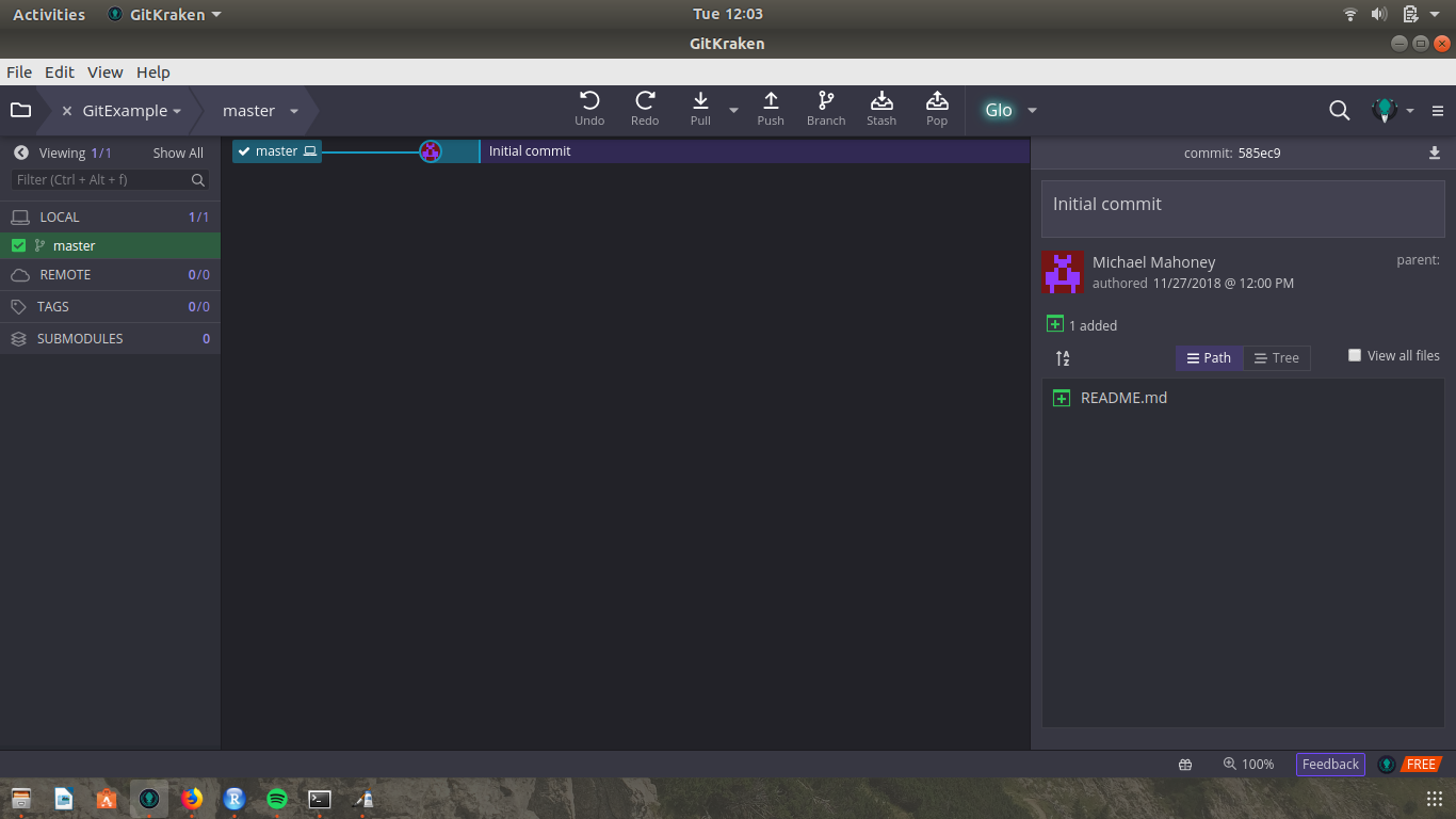
Let’s make a new project R project now through R Studio. We want to create a project in an existing directory, and select our repository as the folder to create the project in.
Once your new project has loaded, open a new script file (Ctrl/Cmd+Shift+N) and type in the following code:
library(tidyverse)
ggplot(iris, aes(Sepal.Length, Sepal.Width)) +
  geom_point()
We should know what this code will give us by now - the same iris scatterplot we’ve been working with for most of this reader.
Save your script using whatever name makes sense to you (I went with Scatterplot.R). If we open GitKraken now, we should see a screen that looks like this:
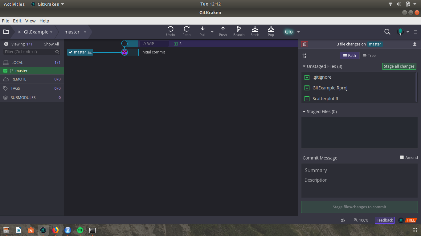
You’ll notice that the left-hand side of the screen has changed, and our new files are listed as “unstaged” changes. To understand what this means, let’s back up a little and talk about what a Git workflow looks like:
10.3.1.1 Commits
The most recent version of your code - the one that anyone with access to your repository should see, that works and is up-to-date - is what’s known as your most recent commit. Commits are versions of the code where you’ve decided to confirm that you like your changes, and want to save them in your project’s development history.
In order to do that, you have to be very specific in telling Git which files you want to include in that commit. Git keeps track of every file you’ve changed since your last commit, and will include them in that “Unstaged Files” window you see our files in. For those changes to be saved, however, we need to stage our changes, and then commit them. GitKraken makes that easy enough - we just click “Stage All Changes”, add a commit message, and then click “Commit Changes”.
A note on commit messages, by the way - these are the main ways you’ll identify what each change actually did to your code when you’re looking at the history, and will be super important if you have to revert to a prior state! As such, try and keep each commit message short but explanatory - “did stuff” is much less helpful than “model selection algorithim now supports AIC”, for instance!
On a similar note, you should commit whenever it makes sense to you to do so - when your code is in a place you may want to get back to. Generally this means that whatever you’ve written works, or is very close to working, or was enough effort to do that you don’t want to bother retyping it should you accidentally break it. There isn’t a hard and fast rule as to when you should commit - but the general rule is “early and often”.
Anyway, go ahead and commit all your changes now. Personally, my message was “made the base scatterplot”.
10.3.1.2 Branches
In the top bar of GitKraken, you should notice a button labeled “branch”. Clicking this will open a box that tells you to “enter branch name”. Right now, I’m naming this branch redplot.
A “branch” is a copy of the code at the time that it’s created - so it “branches” off of the master code (sometimes referred to as the “trunk”). This way, multiple people can work on different parts of the project at the same time - and if you leave an idea half-baked for a while, it won’t disturb the main body of code. GitHub has a nice explanation of how branches work here, if you want more detail.
Now that we’re working in the redplot branch, let’s change our code so that the points are red:
library(tidyverse)
ggplot(iris, aes(Sepal.Length, Sepal.Width)) +
  geom_point(color = "red")
We can now commit this change to our branch, updating the code there without disturbing the code in the master branch. Let’s do this now!
You’ll notice now that you have two labels to your commit messages - master and redplot. If we’ve decided we like our plots red, we can merge the branch into the trunk by right clicking on master and selecting “merge redplot into master”.
Tada! Our branches have merged, our change to the code has become incorporated in the master repository, and we’re understanding the basics of Git. The only thing left to do in this unit is to talk about working with GitHub.
10.3.1.3 Push + Pull
Again, GitHub is an online service which makes working with others using Git much easier than most other services. It will host your repositories online and let others access them.
To do that, we first have to make an online repository. Log into GitHub (or create an account, if you still haven’t) and then click the “+” sign next to your profile photo, then click “New Repository”. Give a name that makes sense (I chose “GitExample”) and don’t check any boxes, then click “Create Repository”. Copy the URL inside the blue box (labeled “Quick Setup”).
Then, in GitKraken, hover over the “0/0” displayed next to “Remote” and click the “+” sign that appears. Type your repository’s name into the “Name” field, then paste the URL into the “Pull URL” field. Once you click “add remote” you’ll be connected to your online repository!
We can now upload our code to this repository, using the “Push” button (located next to “Branch”) and then clicking “Submit”. Your code is now online (reload the GitHub page to see it), and accessible by collaborators! This is called “pushing” your code, and is the next step up from commits - if you’re committing early and often, you should be pushing every time you’ve got something new that works.
The other side of “pushing” is “pulling”, done through the “pull” button in the top bar. If your collaborators have pushed code that impacts your work, you should make sure to pull it to your machine - otherwise, you might be introducing bugs into the system!
This is a super basic introduction to Git, but should be enough to get you started using version control on your own projects. Once you do, it becomes much, MUCH easier to interact with other developers, and to collaborate on projects with people working anywhere in the world.
10.4 Commenting Code
Commenting your code is like cleaning your bathroom - you never want to do it, but it really does create a more pleasant experience for you and your guests.— Ryan Campbell
When you insert a hashtag (#) before a line in your code, R won’t try to run it. This can be used to explain what you’re doing at each step of a complicated process, and is referred to as commenting your code. For instance:
## Comments like this usually explain the purpose of a block of code
ggplot(iris, aes(Sepal.Length, Sepal.Width)) +
  geom_point() # Whereas comments like this usually explain a specific line
It’s a best practice to continuously comment your code - both so that any collaborators you may have can understand what you’ve done, and so that you understand your own work when you come back to it in the future. However, you shouldn’t write comments only explaining what your code does - everyone touching your project should be able to understand that. Instead, good comments explain why you’re doing a particular thing - what your end goal and motivations for each step of the process are, so that others can follow your line of thinking.
10.5 Further Reading
I had originally planned to write a section of this chapter on the basics of making R packages, in order to quickly and easily share functions and code with a wide variety of people. However, I think that may be slightly outside of the scope of this introduction level text - and there’s already a very good textbook on the subject written by people far more qualified than I. For a full explanation of why (and, to an extent, how) you should build packages, check out the Leek Group guide to developing R packages.
Additionally, if you’re interested in getting further into Git, check out Pro Git available for free online.