Chapter 4 Lab 2 - 15/10/2021

In this lecture we will learn to import data from a comma-separated (csv) file, to explore data frames and to compute returns.

4.1 Data import

We have some financial data (i.e. prices) available in the csv file named Adjcloseprices.csv. Note that a csv file can be open using a text editor (e.g. TextNote, TextEdit), see Figure 4.1.

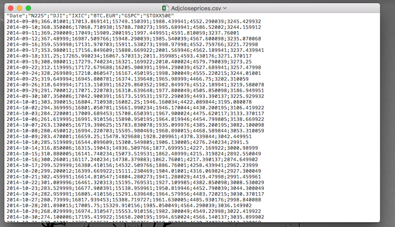
Figure 4.1: Preview of the Adjcloseprices.csv file

There are 3 things that characterize a csv file:

the header: the first line containing the names of the variables;
the field separator (delimiter): the character separating the information (usually the semicolon or the comma is used);
the decimal separator: the character used for real number decimal points (it can be the full stop or the comma).

In the preview of the csv file reported in Figure 4.1

the header is given by a set of text strings:
“;” is the field separator;
“.” is the decimal separator.

All this information are required when importing the data in R by using the read.csv function, whose main arguments are reported here below (see ?read.csv):

file: the name of the file which the data are to be read from; this can also including the specification of the folder path (use quotes to specify it);
header: a logical value (T or F) indicating whether the file contains the names of the variables as its first line;
sep: the field separator character (use quotes to specify it);
dec: the character used in the file for decimal points (use quotes to specify it).

The following code is used to import the data available in the Adjcloseprices.csv file. The output is an object named fdata:

fdata = read.csv("~/Dropbox/UniBg/Didattica/Economia/2021-2022/PSBF_2122/R_LABS/Lab02/Adjcloseprices.csv",header=T,sep=";",dec=".")

The argument header=T and dec="." are set to the default value (see ?read.csv) and they could be omitted.

Alternatively, it is possible to use the user-friendly feature provided by RStudio: read here for more information. The data import feature can be accessed from the environment (top-right) panel (see Figure 4.2). Then all the necessary information can be specified in the following Import Dataset window as shown in Figure 4.3.

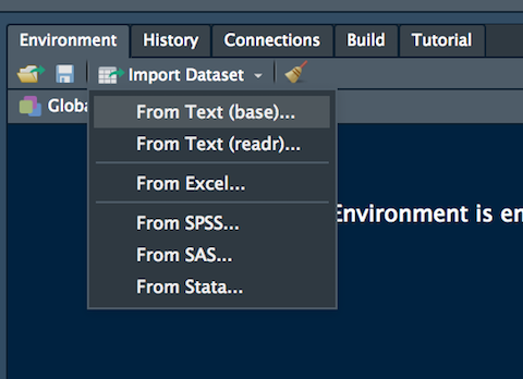
Figure 4.2: The Import Dataset feature of RStudio

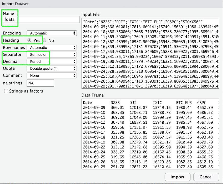
Figure 4.3: Specification of the csv file characteristics through the Import Dataset feature

After clicking on Import an object named fdata will be created (essentially this RStudio feature makes use of the read.csv function).

The fdata is an object of class data.frame:

class(fdata)

## [1] "data.frame"

Data frames are matrix of data where you can find subjects (in this case each day) in the rows and variables in the column (in this case you have the following variables: dates, AAPL prices, etc.).

By using str we get information about the type of variables included in the data frame:

str(fdata)

## 'data.frame':	1008 obs. of  7 variables:
##  $ Date: chr  "2017-09-11" "2017-09-12" "2017-09-13" "2017-09-14" ...
##  $ AAPL: num  38.5 38.4 38.1 37.8 38.1 ...
##  $ GSAT: num  1.6 1.68 1.77 1.78 1.82 1.78 1.77 1.8 1.79 1.77 ...
##  $ AMC : num  11.3 11.4 12.2 12.9 13.6 ...
##  $ AAL : num  44.6 45 45.7 44.9 44.7 ...
##  $ F   : num  9.69 9.85 9.87 9.82 9.87 ...
##  $ IXIC: num  6432 6454 6460 6429 6448 ...

In this case the variable Date is interpreted as a qualitative variable (chr stands for characters, a vector of strings) while the other variables (all the prices) are in the form of numerical variables.

It is possible to get a preview of the top or bottom part of the data frame by using head or tail:

head(fdata) #preview of the first 6 lines (oldest data)

##         Date     AAPL GSAT      AMC      AAL        F    IXIC
## 1 2017-09-11 38.53323 1.60 11.32855 44.60053 9.694755 6432.26
## 2 2017-09-12 38.38054 1.68 11.40889 45.01872 9.847696 6454.28
## 3 2017-09-13 38.09183 1.77 12.21233 45.70923 9.873184 6460.19
## 4 2017-09-14 37.76495 1.78 12.89526 44.92147 9.822205 6429.08
## 5 2017-09-15 38.14671 1.82 13.61836 44.73669 9.873184 6448.47
## 6 2017-09-18 37.85801 1.78 13.37733 44.06564 9.881683 6454.64

tail(fdata) #preview of the last 6 lines (most recent data)

##            Date   AAPL GSAT   AMC   AAL     F     IXIC
## 1003 2021-09-02 153.65 2.10 44.38 19.76 13.01 15331.18
## 1004 2021-09-03 154.30 2.20 44.02 19.37 12.89 15363.52
## 1005 2021-09-07 156.69 2.07 47.83 19.53 12.95 15374.33
## 1006 2021-09-08 155.11 2.69 47.40 19.13 13.03 15286.64
## 1007 2021-09-09 154.07 2.58 48.52 20.20 12.76 15248.25
## 1008 2021-09-10 148.97 2.60 50.16 18.95 12.68 15115.49

Note that the top of the data frame contains the oldest data while the bottom part of the data frame the most recent data.

Use the following alternative function if you want to get information about the dimensions of the data frame:

nrow(fdata) #number of rows

## [1] 1008

ncol(fdata) #number of columns

## [1] 7

dim(fdata) #no. of rows and columns

## [1] 1008    7

4.2 Data selection from a data frame

To select data it is possible to use squared parentheses as seen in Lab 1 for vectors, but in this case two indexes (one for the row and one for the column) will have to be specified. For example the code

fdata[4,4] #first number is the row index, the second is the column index

## [1] 12.89526

is used to retrieve the element in the 4-th row and 4-th column, corresponding to the value of AMC for “2017-09-14”.

If more elements together are requested, a vector of indexes can be used:

fdata[ c(100,101,102) , 4] #rows 100, 101, 102, 4th column

## [1] 11.00088 11.36758 10.87865

# shorter code for the regular sequence  100, 101, 102
fdata[ 100:102 , 4]

## [1] 11.00088 11.36758 10.87865

To select an entire row (i.e. all the prices for a given day) you have to specify only the row index:

fdata[4,] #all the data for the 4th day

##         Date     AAPL GSAT      AMC      AAL        F    IXIC
## 4 2017-09-14 37.76495 1.78 12.89526 44.92147 9.822205 6429.08

Similarly, if you are interested in a particular column (i.e. all the prices for a given asset), specify only the column index

fdata[,4] #all the values (1058) for IXIC

##    [1] 11.328548 11.408892 12.212335 12.895262 13.618361 13.377328 12.573884
##    [8] 12.332852 12.694401 12.774745 12.172163 12.373023 12.453368 12.051645
##   [15] 11.810614 11.810614 12.774745 12.694401 12.895262 12.212335 11.248203
##   [22] 11.127688 11.047342 11.127688 11.047342 11.047342 11.047342 10.926828
##   [29] 11.449065 11.248203 11.368720 11.489236 11.288376 11.810614 11.850787
##   [36] 11.167859 11.167859 10.806310 10.324244  9.560974  9.802007  9.882351
##   [43]  9.480629  9.159251  8.837874  9.360112  9.802007 10.083211 10.002866
##   [50] 10.404589 10.243900 10.203728 10.605451 11.127688 11.971303 12.975606
##   [57] 12.373023 11.449065 11.408320 11.652783 11.775017 11.612041 11.693530
##   [64] 11.937992 12.426921 12.426921 12.345433 12.875105 12.304689 12.426921
##   [71] 12.426921 12.100968 12.549152 12.141713 11.734273 11.489808 12.100968
##   [78] 12.304689 12.549152 12.223200 11.775017 11.489808 11.245345 11.326833
##   [85] 11.367578 11.489808 11.775017 11.123112 11.204602 10.919392 10.756416
##   [92] 10.797159 10.919392 10.756416 10.715673 10.471209 10.471209 10.267489
##   [99] 10.430464 11.000881 11.367578 10.878650 11.204602 11.571296 11.204602
##  [106] 10.960136 11.326833 11.286089 11.612041 11.937992 11.734273 11.815761
##  [113] 11.734273 11.652783 12.100968 12.589896 12.834361 12.223200 12.019481
##  [120] 12.834361 12.834361 12.997338 12.793618 12.671385 12.960310 12.919033
##  [127] 12.176086 12.423735 12.176086 11.722062 11.680789 11.598239 11.680789
##  [134] 11.391865 11.474415 11.515689 11.226765 11.144215 11.598239 11.680789
##  [141] 12.588834 12.712659 13.496881 13.579432 13.579432 13.868354 13.785807
##  [148] 13.620708 13.992182 14.157281 14.363657 14.487478 14.239828 14.033455
##  [155] 14.157281 14.198557 14.239828 14.198557 14.198557 14.404930 13.538156
##  [162] 13.620708 13.661981 13.455607 14.198557 13.868354 13.249232 13.579432
##  [169] 13.455607 13.538156 13.661981 13.703255 13.703255 13.290507 13.249232
##  [176] 12.877759 12.547560 12.588834 12.423735 11.928435 12.258636 12.217360
##  [183] 12.217360 12.010988 12.176086 12.134812 12.093535 12.093535 12.511998
##  [190] 13.097843 12.930459 13.181537 13.055998 13.390767 13.599998 13.892920
##  [197] 14.395074 13.892920 13.809229 13.265228 13.055998 13.516304 13.307075
##  [204] 13.181537 13.265228 14.060305 14.478766 14.353227 14.520614 14.562457
##  [211] 14.227690 14.269536 13.976613 14.102152 13.683691 13.767382 13.348920
##  [218] 13.014152 12.972306 12.763074 13.139690 13.139690 12.846766 13.641843
##  [225] 13.432612 13.851074 14.353227 14.478766 14.395074 14.646152 14.143997
##  [232] 14.604307 14.604307 14.646152 14.813537 15.148305 15.357535 15.524919
##  [239] 15.775999 15.901537 16.068920 16.027073 15.650459 16.027073 15.859691
##  [246] 15.734150 15.943381 16.110767 16.152615 16.529230 16.825148 16.825148
##  [253] 16.740601 16.951971 16.994246 16.740601 16.867422 16.909695 17.459259
##  [260] 17.543808 18.051102 18.598103 18.142267 18.370186 18.643690 18.689270
##  [267] 18.105803 18.014633 18.315487 18.206083 17.959932 17.868767 17.877882
##  [274] 17.093845 16.783878 17.194130 17.567915 18.370186 18.060219 17.905231
##  [281] 18.060219 18.051102 17.959932 16.255108 17.057379 16.255108 17.066492
##  [288] 17.540565 17.558798 17.540565 17.321762 17.485865 16.792994 16.756523
##  [295] 16.528606 14.276779 13.848293 14.167378 14.295013 13.438041 12.808987
##  [302] 12.298451 12.116117 12.708704 12.654004 12.909272 12.261984 12.617537
##  [309] 12.726937 12.444319 12.963973 13.000439 13.337758 13.189869 13.217599
##  [316] 13.975531 14.114176 13.735209 13.411703 13.005007 12.903334 12.357991
##  [323] 11.997512 11.405956 11.332010 11.720221 11.276552 11.479900 11.350496
##  [330] 11.914326 12.071457 12.515124 13.051224 13.467159 12.894091 12.690743
##  [337] 12.968036 13.060465 13.226841 13.032737 13.041979 13.365488 12.487394
##  [344] 12.746201 13.171384 12.949550 12.949550 13.115924 13.051224 13.541105
##  [351] 13.115924 13.263814 13.005007 12.746201 12.311776 12.681499 12.173131
##  [358] 12.256317 12.487394 12.616798 12.746201 12.200859 12.635283 12.663014
##  [365] 12.820147 12.607554 12.533610 12.820147 12.968036 14.788920 14.326768
##  [372] 14.437683 13.984773 13.679752 13.792188 13.726600 13.511098 13.520467
##  [379] 13.567315 13.586055 14.054539 13.820297 14.017061 14.448067 14.110758
##  [386] 14.335630 13.998321 13.904624 13.839037 13.913995 14.045170 13.848406
##  [393] 13.689121 14.063910 14.035799 15.281968 15.132053 15.132053 15.103945
##  [400] 15.394405 15.459993 15.544322 15.544322 15.038357 14.298152 14.288780
##  [407] 14.466805 14.335630 14.429327 14.523025 14.204454 13.782819 13.773447
##  [414] 13.670382 13.932733 14.026430 13.726600 12.770891 12.948915 12.452321
##  [421] 12.649085 12.724042 12.555388 12.302406 12.180601 12.377365 12.218080
##  [428] 12.133752 11.890139 11.712117 11.299850 11.253001 11.224891 11.149934
##  [435] 11.037498 10.475316 10.390989 10.257404 10.438698 10.534116 10.200154
##  [442] 10.448240 10.457782 10.667701 10.887162 11.001663 10.429156 10.114279
##  [449]  9.551314  9.045600  9.016974  9.055141  8.902473  8.845223  8.787971
##  [456]  8.683013  8.969265  8.454010  8.501719  8.797514  9.016974  9.026517
##  [463]  9.055141  9.331853  9.360478  9.179185 10.057028  9.932984  9.828026
##  [470] 10.286029 10.438698 10.734493 10.925329 11.202041 11.287916 10.744036
##  [477] 11.087539 10.591367 10.801286 10.829910 11.459668 11.621879 11.221124
##  [484] 11.135247 10.257404 10.343281 10.639075 10.868079 10.820370 10.887162
##  [491] 10.982579 10.505490 10.791744 10.362364 10.734493 10.782202 10.600909
##  [498] 10.877620 11.173415 11.469211 11.178113 11.333365 11.304255 11.391583
##  [505] 11.352771 11.605055 11.556539 11.149003 10.838500 10.450372 10.527998
##  [512] 10.401855 10.392153 10.489184 10.498887 10.460074 10.382448 10.304823
##  [519]  9.916694  9.635301  9.528564  9.489753  9.538269  9.111327  8.888152
##  [526]  8.946372  8.684385  8.897856  9.062810  9.062810  9.082216  8.946372
##  [533]  9.470345  9.577082  9.315094  9.431533  9.615893  9.518862  9.121030
##  [540]  9.091920  9.334500  9.460643  9.489753  9.402422  8.965777  9.334500
##  [547]  9.256875  9.004591  8.538836  8.616463  8.500024  8.218631  8.218631
##  [554]  7.888721  7.704359  7.723765  8.131302  7.665546  8.179817  8.130122
##  [561]  8.617134  8.219574  7.881646  7.822012  8.000915  8.179816  8.050611
##  [568]  8.110244  8.249391  8.169878  8.299086  8.070488  7.911463  7.752439
##  [575]  7.682866  7.275366  7.464208  7.295244  7.255488  7.195854  7.195854
##  [582]  7.414512  7.275366  7.076585  7.086524  6.579634  6.420610  6.430549
##  [589]  6.520000  6.808232  7.066647  7.285305  7.235610  7.136220  6.927500
##  [596]  6.758537  6.698902  6.321219  6.748598  6.728720  6.798293  6.480244
##  [603]  6.410671  6.609451  6.957317  6.708841  6.510061  6.748598  6.897683
##  [610]  6.818171  6.957317  7.056707  6.997073  7.265427  7.712683  7.414512
##  [617]  7.007012  6.510061  5.893841  6.052866  6.221829  6.072744  5.774573
##  [624]  5.784513  4.890000  4.530000  3.850000  4.200000  3.640000  2.910000
##  [631]  3.220000  2.600000  2.480000  2.470000  3.370000  3.190000  3.150000
##  [638]  3.560000  3.460000  3.700000  3.600000  3.040000  3.160000  2.620000
##  [645]  2.240000  2.270000  2.880000  3.140000  3.300000  2.600000  2.080000
##  [652]  2.180000  2.410000  2.440000  3.200000  3.180000  3.250000  3.180000
##  [659]  3.110000  3.050000  3.360000  4.140000  5.190000  4.920000  4.570000
##  [666]  4.300000  3.890000  3.920000  3.990000  4.100000  5.320000  5.120000
##  [673]  4.600000  4.550000  4.520000  4.720000  4.560000  4.660000  4.630000
##  [680]  4.580000  5.110000  5.600000  5.070000  5.130000  5.310000  5.590000
##  [687]  5.450000  5.380000  5.910000  6.450000  5.990000  6.290000  5.170000
##  [694]  5.890000  5.800000  5.560000  5.420000  5.630000  5.520000  5.330000
##  [701]  5.100000  4.790000  4.270000  4.180000  4.420000  4.290000  4.570000
##  [708]  4.530000  4.280000  4.130000  4.430000  4.570000  4.600000  4.260000
##  [715]  4.220000  4.500000  4.380000  4.270000  4.150000  4.150000  4.030000
##  [722]  4.060000  4.000000  3.870000  4.150000  4.160000  4.120000  4.040000
##  [729]  4.110000  4.100000  4.150000  4.140000  4.750000  4.470000  4.560000
##  [736]  4.640000  5.310000  5.540000  5.600000  5.350000  5.390000  5.690000
##  [743]  5.190000  5.410000  5.540000  5.600000  6.520000  6.300000  5.880000
##  [750]  6.070000  7.040000  6.600000  7.020000  6.420000  6.260000  5.940000
##  [757]  5.790000  5.540000  5.520000  5.760000  5.720000  5.670000  5.320000
##  [764]  5.210000  4.780000  4.610000  4.880000  4.910000  4.860000  4.710000
##  [771]  4.650000  4.650000  4.130000  4.060000  4.040000  4.140000  4.050000
##  [778]  4.080000  3.540000  2.960000  2.780000  3.040000  3.540000  3.090000
##  [785]  3.000000  3.120000  2.970000  2.750000  2.790000  2.610000  2.520000
##  [792]  2.360000  2.150000  2.340000  2.310000  2.460000  2.490000  3.770000
##  [799]  3.510000  3.130000  2.940000  2.970000  3.110000  2.980000  3.260000
##  [806]  3.190000  3.350000  3.810000  4.580000  4.490000  4.450000  4.270000
##  [813]  4.150000  4.320000  3.630000  3.510000  3.560000  3.980000  3.860000
##  [820]  4.090000  3.920000  3.190000  2.860000  2.780000  2.850000  2.800000
##  [827]  2.680000  2.590000  2.560000  2.510000  2.390000  2.290000  2.160000
##  [834]  2.120000  2.010000  1.980000  2.010000  2.050000  2.140000  2.200000
##  [841]  2.290000  2.180000  2.180000  2.330000  3.060000  2.970000  2.980000
##  [848]  3.510000  4.420000  4.960000 19.900000  8.630000 13.260000 13.300000
##  [855]  7.820000  8.970000  7.090000  6.830000  6.180000  5.500000  5.800000
##  [862]  5.610000  5.590000  5.650000  5.550000  5.510000  5.700000  6.550000
##  [869]  7.700000  9.090000  8.290000  8.010000  9.180000  8.930000  8.580000
##  [876]  8.030000  8.050000  9.290000 10.500000  9.850000 10.280000 11.160000
##  [883] 14.040000 13.020000 13.560000 14.000000 13.930000 12.490000 10.660000
##  [890]  9.020000 10.940000 10.240000 10.350000 10.350000 10.210000  9.360000
##  [897] 10.610000 10.200000  9.850000  9.790000  9.420000  8.620000  8.840000
##  [904]  9.350000  9.900000  9.330000  9.660000  9.280000  9.780000  9.990000
##  [911] 10.160000 11.500000 11.460000 10.850000 10.200000 10.030000  9.710000
##  [918]  9.390000  9.170000  9.000000  9.510000  9.740000 10.050000 10.320000
##  [925] 12.770000 12.980000 13.950000 14.030000 12.640000 12.550000 12.080000
##  [932] 13.680000 16.410000 19.559999 26.520000 26.120001 32.040001 62.549999
##  [939] 51.340000 47.910000 55.000000 55.049999 49.340000 42.810001 49.400002
##  [946] 57.000000 59.040001 55.180000 60.730000 59.259998 55.689999 58.270000
##  [953] 58.299999 56.700001 54.060001 58.110001 56.430000 56.680000 54.220001
##  [960] 51.959999 49.959999 45.070000 47.939999 46.189999 42.610001 39.349998
##  [967] 33.430000 36.000000 34.959999 34.619999 43.090000 40.779999 37.240002
##  [974] 36.990002 40.290001 38.009998 38.900002 38.130001 37.020000 35.200001
##  [981] 33.590000 29.840000 33.509998 32.700001 33.799999 31.750000 31.549999
##  [988] 33.070000 33.470001 35.689999 37.160000 36.549999 33.820000 34.410000
##  [995] 36.779999 44.259998 43.959999 40.310001 40.840000 43.330002 47.130001
## [1002] 43.689999 44.380001 44.020000 47.830002 47.400002 48.520000 50.160000

or alternatively perform the selection by using the $ followed by the column name:

fdata$IXIC #this is a vector (one dimensional object)

##    [1]  6432.26  6454.28  6460.19  6429.08  6448.47  6454.64  6461.32  6456.04
##    [9]  6422.69  6426.92  6370.59  6380.16  6453.26  6453.45  6495.96  6516.72
##   [17]  6531.71  6534.63  6585.36  6590.18  6579.73  6587.25  6603.55  6591.51
##   [25]  6605.80  6624.00  6623.66  6624.22  6605.07  6629.05  6586.83  6598.43
##   [33]  6563.89  6556.77  6701.26  6698.96  6727.67  6716.53  6714.94  6764.44
##   [41]  6786.44  6767.78  6789.12  6750.05  6750.94  6757.60  6737.87  6706.21
##   [49]  6793.29  6782.79  6790.71  6862.48  6867.36  6889.16  6878.52  6912.36
##   [57]  6824.39  6873.97  6847.59  6775.37  6762.21  6776.38  6812.84  6840.08
##   [65]  6875.08  6862.32  6875.80  6856.53  6936.58  6994.76  6963.85  6960.96
##   [73]  6965.36  6959.96  6936.25  6939.34  6950.16  6903.39  7006.90  7065.53
##   [81]  7077.91  7136.56  7157.39  7163.58  7153.57  7211.78  7261.06  7223.69
##   [89]  7298.28  7296.05  7336.38  7408.03  7460.29  7415.06  7411.16  7505.77
##   [97]  7466.51  7402.48  7411.48  7385.86  7240.95  6967.53  7115.88  7051.98
##  [105]  6777.16  6874.49  6981.96  7013.51  7143.62  7256.43  7239.47  7234.31
##  [113]  7218.23  7210.09  7337.39  7421.46  7330.35  7273.01  7180.56  7257.87
##  [121]  7330.71  7372.01  7396.65  7427.95  7560.81  7588.32  7511.01  7496.81
##  [129]  7481.74  7481.99  7344.24  7364.30  7345.29  7166.68  6992.67  7220.54
##  [137]  7008.81  6949.23  7063.45  6870.12  6941.28  7042.11  7076.55  6915.11
##  [145]  6950.34  7094.30  7069.03  7140.25  7106.65  7156.28  7281.10  7295.24
##  [153]  7238.06  7146.13  7128.60  7007.35  7003.74  7118.68  7119.80  7066.27
##  [161]  7130.70  7100.90  7088.15  7209.62  7265.21  7266.90  7339.91  7404.97
##  [169]  7402.88  7411.32  7351.63  7398.30  7382.47  7354.34  7394.04  7378.46
##  [177]  7425.96  7424.43  7433.85  7396.59  7462.45  7442.12  7554.33  7606.46
##  [185]  7637.86  7689.24  7635.07  7645.51  7659.93  7703.79  7695.70  7761.04
##  [193]  7746.38  7747.03  7725.59  7781.51  7712.95  7692.82  7532.01  7561.63
##  [201]  7445.08  7503.68  7510.30  7567.69  7502.67  7586.43  7688.39  7756.20
##  [209]  7759.20  7716.61  7823.92  7825.98  7805.72  7855.12  7854.44  7825.30
##  [217]  7820.20  7841.87  7840.77  7932.24  7852.18  7737.42  7630.00  7671.79
##  [225]  7707.29  7802.69  7812.01  7859.68  7883.66  7888.33  7891.78  7839.11
##  [233]  7819.71  7870.89  7774.12  7806.52  7816.33  7821.01  7859.17  7889.10
##  [241]  7878.46  7945.98  8017.90  8030.04  8109.69  8088.36  8109.54  8091.25
##  [249]  7995.17  7922.73  7902.54  7924.16  7972.47  7954.23  8013.71  8010.04
##  [257]  7895.79  7956.11  7950.04  8028.23  7986.96  7993.25  8007.47  7990.37
##  [265]  8041.97  8046.35  8037.30  7999.55  8025.09  7879.51  7788.45  7735.95
##  [273]  7738.02  7422.05  7329.06  7496.89  7430.74  7645.49  7642.70  7485.14
##  [281]  7449.03  7468.63  7437.54  7108.40  7318.34  7167.21  7050.29  7161.65
##  [289]  7305.90  7434.06  7356.99  7328.85  7375.96  7570.75  7530.88  7406.90
##  [297]  7200.87  7200.87  7136.39  7259.03  7247.87  7028.48  6908.82  6972.25
##  [305]  6938.98  7081.85  7082.70  7291.59  7273.08  7330.54  7441.51  7158.43
##  [313]  7188.26  6969.25  7020.52  7031.83  7098.31  7070.33  6910.66  6753.73
##  [321]  6783.91  6636.83  6528.41  6332.99  6192.92  6554.36  6579.49  6584.52
##  [329]  6635.28  6665.94  6463.50  6738.86  6823.47  6897.00  6957.08  6986.07
##  [337]  6971.48  6905.92  7023.83  7034.69  7084.46  7157.23  7020.36  7025.77
##  [345]  7073.46  7164.86  7085.68  7028.29  7183.08  7281.74  7263.87  7347.54
##  [353]  7402.08  7375.28  7288.35  7298.20  7307.90  7414.62  7420.38  7426.95
##  [361]  7472.41  7486.77  7489.07  7459.71  7527.54  7554.46  7549.30  7554.51
##  [369]  7532.53  7595.35  7577.57  7576.36  7505.92  7421.46  7408.14  7558.06
##  [377]  7591.03  7643.41  7630.91  7688.53  7714.48  7723.95  7728.97  7838.96
##  [385]  7642.67  7637.54  7691.52  7643.38  7669.17  7729.32  7828.91  7848.69
##  [393]  7895.55  7891.78  7938.69  7953.88  7909.28  7964.24  7947.36  7984.16
##  [401]  7976.01  8000.23  7996.08  7998.06  8015.27  8120.82  8102.01  8118.68
##  [409]  8146.40  8161.85  8095.39  8049.64  8036.77  8164.00  8123.29  7963.76
##  [417]  7943.32  7910.59  7916.94  7647.02  7734.49  7822.15  7898.05  7816.28
##  [425]  7702.38  7785.72  7750.84  7628.28  7637.01  7607.35  7547.31  7567.72
##  [433]  7453.15  7333.02  7527.12  7575.48  7615.55  7742.10  7823.17  7822.57
##  [441]  7792.72  7837.13  7796.66  7845.02  7953.88  7987.32  8051.34  8031.71
##  [449]  8005.70  7884.72  7909.97  7967.76  8006.24  8091.16  8109.09  8170.23
##  [457]  8161.79  8098.38  8141.73  8202.53  8196.04  8244.14  8258.19  8222.80
##  [465]  8185.21  8207.24  8146.49  8204.14  8251.40  8321.50  8238.54  8330.21
##  [473]  8293.33  8273.61  8175.42  8111.12  8004.07  7726.04  7833.27  7862.83
##  [481]  8039.16  7959.14  7863.41  8016.36  7773.94  7766.62  7895.99  8002.81
##  [489]  7948.56  8020.21  7991.39  7751.77  7853.74  7826.95  7856.88  7973.39
##  [497]  7962.88  7874.16  7976.88  8116.83  8103.07  8087.44  8084.16  8169.68
##  [505]  8194.47  8176.71  8153.54  8186.02  8177.39  8182.88  8117.67  8112.46
##  [513]  7993.63  8077.38  8030.66  7939.63  7999.34  7908.68  7785.25  7872.26
##  [521]  7982.47  7956.29  7823.78  7903.74  7950.78  8057.04  8048.65  8148.71
##  [529]  8124.18  8156.85  8089.54  8162.99  8104.30  8119.79  8185.80  8243.12
##  [537]  8325.99  8276.85  8303.98  8292.36  8386.40  8433.20  8434.68  8410.63
##  [545]  8434.52  8475.31  8464.28  8486.09  8482.10  8479.02  8540.83  8549.94
##  [553]  8570.66  8526.73  8506.21  8519.88  8632.49  8647.93  8705.18  8665.47
##  [561]  8567.99  8520.64  8566.67  8570.70  8656.53  8621.83  8616.18  8654.05
##  [569]  8717.32  8734.88  8814.23  8823.36  8827.74  8887.22  8924.96  8945.65
##  [577]  8952.88  9022.39  9006.62  8945.99  8972.60  9092.19  9020.77  9071.47
##  [585]  9068.58  9129.24  9203.43  9178.86  9273.93  9251.33  9258.70  9357.13
##  [593]  9388.94  9370.81  9383.77  9402.48  9314.91  9139.31  9269.68  9275.16
##  [601]  9298.93  9150.94  9273.40  9467.97  9508.68  9572.15  9520.51  9628.39
##  [609]  9638.94  9725.96  9711.97  9731.18  9732.74  9817.18  9750.97  9576.59
##  [617]  9221.28  8965.61  8980.78  8566.48  8567.37  8952.17  8684.09  9018.09
##  [625]  8738.59  8575.62  7950.68  8344.25  7952.05  7201.80  7874.88  6904.59
##  [633]  7334.78  6989.84  7150.58  6879.52  6860.67  7417.86  7384.30  7797.54
##  [641]  7502.38  7774.15  7700.10  7360.58  7487.31  7373.08  7913.24  7887.26
##  [649]  8090.90  8153.58  8192.42  8515.74  8393.18  8532.36  8650.14  8560.73
##  [657]  8263.23  8495.38  8494.75  8634.52  8730.16  8607.73  8914.71  8889.55
##  [665]  8604.95  8710.71  8809.12  8854.39  8979.66  9121.32  9192.34  9002.55
##  [673]  8863.17  8943.72  9014.56  9234.83  9185.10  9375.78  9284.88  9324.59
##  [681]  9340.22  9412.36  9368.99  9489.87  9552.05  9608.38  9682.91  9615.81
##  [689]  9814.08  9924.75  9953.75 10020.35  9492.73  9588.81  9726.02  9895.87
##  [697]  9910.53  9943.05  9946.12 10056.48 10131.37  9909.17 10017.00  9757.22
##  [705]  9874.15 10058.77 10154.63 10207.63 10433.65 10343.89 10492.50 10547.75
##  [713] 10617.44 10390.84 10488.58 10550.49 10473.83 10503.19 10767.09 10680.36
##  [721] 10706.13 10461.42 10363.18 10536.27 10402.09 10542.94 10587.81 10745.27
##  [729] 10902.80 10941.17 10998.40 11108.07 11010.98 10968.36 10782.82 11012.24
##  [737] 11042.50 11019.30 11129.73 11210.84 11146.46 11264.95 11311.80 11379.72
##  [745] 11466.47 11665.06 11625.34 11695.63 11775.46 11939.67 12056.44 11458.10
##  [753] 11313.13 10847.69 11141.56 10919.59 10853.55 11056.65 11190.32 11050.47
##  [761] 10910.28 10793.28 10778.80 10963.64 10632.99 10672.27 10913.56 11117.53
##  [769] 11085.25 11167.51 11326.51 11075.02 11332.49 11154.60 11364.60 11420.98
##  [777] 11579.94 11876.26 11863.90 11768.73 11713.87 11671.56 11478.88 11516.49
##  [785] 11484.69 11506.01 11548.28 11358.94 11431.35 11004.87 11185.59 10911.59
##  [793] 10957.61 11160.57 11590.78 11890.93 11895.23 11713.78 11553.86 11786.43
##  [801] 11709.59 11829.29 11924.13 11899.34 11801.60 11904.71 11854.97 11880.63
##  [809] 12036.79 12094.40 12205.85 12198.74 12355.11 12349.37 12377.18 12464.23
##  [817] 12519.95 12582.77 12338.95 12405.81 12377.87 12440.04 12595.06 12658.19
##  [825] 12764.75 12755.64 12742.52 12807.92 12771.11 12804.73 12899.42 12850.22
##  [833] 12870.00 12888.28 12698.45 12818.96 12740.79 13067.48 13201.98 13036.43
##  [841] 13072.43 13128.95 13112.64 12998.50 13197.18 13457.25 13530.91 13543.06
##  [849] 13635.99 13626.06 13270.60 13337.16 13070.69 13403.39 13612.78 13610.54
##  [857] 13777.74 13856.30 13987.64 14007.70 13972.53 14025.77 14095.47 14047.50
##  [865] 13965.49 13865.36 13874.46 13533.05 13465.20 13597.97 13119.43 13192.35
##  [873] 13588.83 13358.79 12997.75 12723.47 12920.15 12609.16 13073.82 13068.83
##  [881] 13398.67 13319.86 13459.71 13471.57 13525.20 13116.17 13215.24 13377.54
##  [889] 13227.70 12961.89 12977.68 13138.73 13059.65 13045.39 13246.87 13480.11
##  [897] 13705.59 13698.38 13688.84 13829.31 13900.19 13850.00 13996.10 13857.84
##  [905] 14038.76 14052.34 13914.77 13786.27 13950.22 13818.41 14016.81 14138.78
##  [913] 14090.22 14051.03 14082.55 13962.68 13895.12 13633.50 13582.42 13632.84
##  [921] 13752.24 13401.86 13389.43 13031.68 13124.99 13429.98 13379.05 13303.64
##  [929] 13299.74 13535.74 13470.99 13661.17 13657.17 13738.00 13736.28 13748.74
##  [937] 13736.48 13756.33 13614.51 13814.49 13881.72 13924.91 13911.75 14020.33
##  [945] 14069.42 14174.14 14072.86 14039.68 14161.35 14030.38 14141.48 14253.27
##  [953] 14271.73 14369.71 14360.39 14500.51 14528.33 14503.95 14522.38 14639.33
##  [961] 14663.64 14665.06 14559.78 14701.92 14733.24 14677.65 14644.95 14543.13
##  [969] 14427.24 14274.98 14498.88 14631.95 14684.60 14836.99 14840.71 14660.58
##  [977] 14762.58 14778.26 14672.68 14681.07 14761.29 14780.53 14895.12 14835.76
##  [985] 14860.18 14788.09 14765.14 14816.26 14822.90 14793.76 14656.18 14525.91
##  [993] 14541.79 14714.66 14942.65 15019.80 15041.86 14945.81 15129.50 15265.89
## [1001] 15259.24 15309.38 15331.18 15363.52 15374.33 15286.64 15248.25 15115.49

Given a vector it is then possible to select an element by using the one dimensional index. Select for example the first value of the vector fdata$IXIC:

fdata$IXIC[1]

## [1] 6432.26

This is equivalent to

fdata[1,7]

## [1] 6432.26

4.3 Exploratory data analysis

Given a vector of data the function summary returns the main summary statistics:

x = fdata$AAPL
summary(x)

##    Min. 1st Qu.  Median    Mean 3rd Qu.    Max. 
##   34.56   44.60   54.49   74.07  113.95  156.69

The summary function returns several summary statistica: min, quartiles, mean and max.

Variability information are missing. They can be obtained by using the var and sd functions:

var(x)

## [1] 1316.017

sd(x)

## [1] 36.27694

If we are interested in getting some summary statistics for all the assets we could use many times the summary function (one for each column). This could be not convenient if you have many columns in your data frame. Alternatively it is possible to use the function apply that makes it possible to use just one line of code for computing the summary statistics jointly for all the columns. Actually we would like to remove the first column containing dates coded as characters. To do this we use the following code:

fdata2 = fdata[,-1] 
#all the rows, all the columns but the first one
str(fdata2)

## 'data.frame':	1008 obs. of  6 variables:
##  $ AAPL: num  38.5 38.4 38.1 37.8 38.1 ...
##  $ GSAT: num  1.6 1.68 1.77 1.78 1.82 1.78 1.77 1.8 1.79 1.77 ...
##  $ AMC : num  11.3 11.4 12.2 12.9 13.6 ...
##  $ AAL : num  44.6 45 45.7 44.9 44.7 ...
##  $ F   : num  9.69 9.85 9.87 9.82 9.87 ...
##  $ IXIC: num  6432 6454 6460 6429 6448 ...

Given fdata2 we want to compute the mean for each column with a single command by using the apply function (see ?apply):

apply(fdata2, 2, mean)

##         AAPL         GSAT          AMC          AAL            F         IXIC 
##   74.0669685    0.7280952   12.3747869   29.1990895    9.3049330 9321.7951530

The second input of the apply function is the MARGIN option. It is equal to 2 if you want to compute the summary statistics column by column. Otherwise it can be 1 if you want to do the computation row by row.

It is also possible to use summary instead of mean:

apply(fdata2, 2, summary)

##              AAPL      GSAT      AMC      AAL         F      IXIC
## Min.     34.55908 0.2600000  1.98000  9.04000  4.010000  6192.920
## 1st Qu.  44.60330 0.3800000  6.72375 19.13750  8.151981  7421.190
## Median   54.49336 0.5000000 11.15497 28.83054  9.074938  8090.220
## Mean     74.06697 0.7280952 12.37479 29.19909  9.304933  9321.795
## 3rd Qu. 113.94959 1.0500000 13.53816 37.44951 10.324820 11120.580
## Max.    156.69000 2.6900000 62.55000 56.98873 15.990000 15374.330

4.4 Graphical representation of the time series

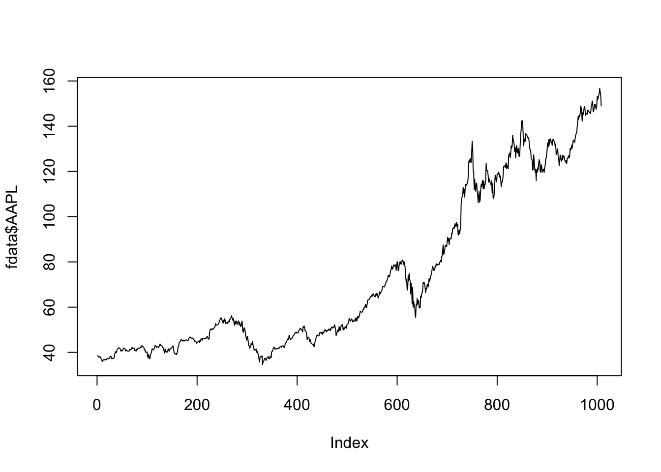
The aim is to plot the price time series for the available assets. We will have a plot with dates on the x-axis and prices on the y-axis. Let’s start by plotting AAPL:

plot(fdata$AAPL)

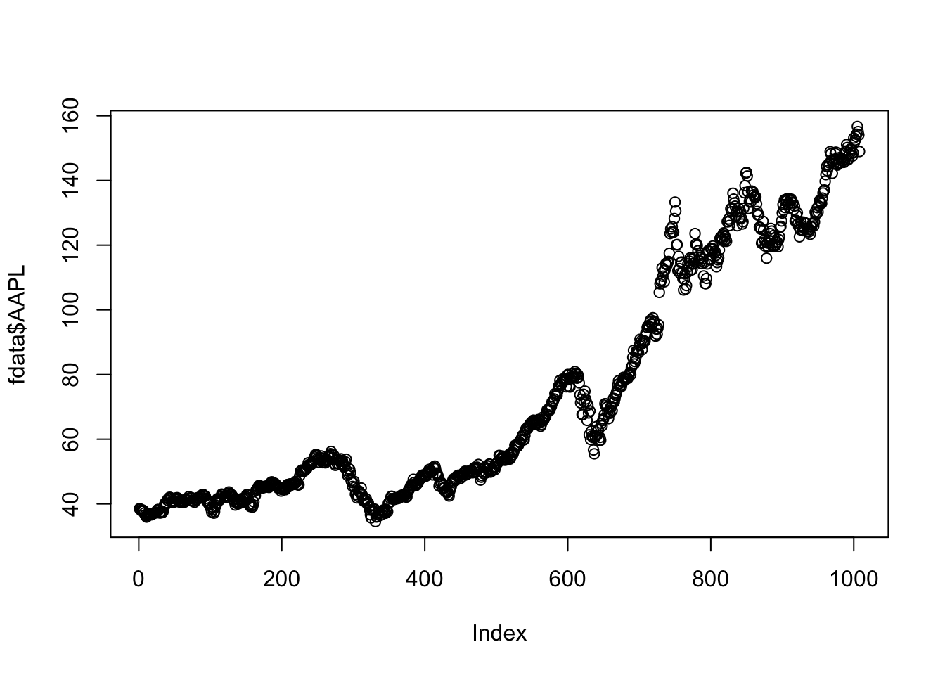Each point represents a day and the level of the point is given by the corresponding price. Note that for the moment on the x-axis by default we have the Index variable going from 1 to the length of the vector (in this case 1008). Having points is not the best choice for representing time series because the temporal evolution of prices is not completely clear. The following code uses the option type="l" (“l” stands for “line”) in order to use a line (instead of points, which is the default setting) for representing the time series.

plot(fdata$AAPL,type="l")

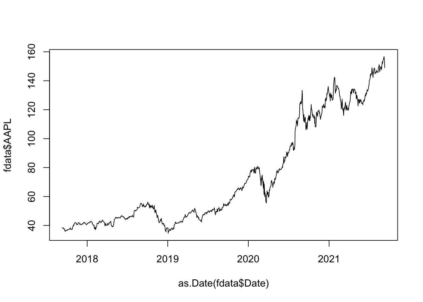
We now want to include dates on the x-axis (this will help in understanding when particular changes in the temporal evolution occur). To do this we need to specify two vectors in the plot function (the vector of dates and the vector of prices). In particular we will apply the as.Date function to fdata$Date in order to transform the vector of characters (remember the output of str) into a vector of proper dates:

plot(as.Date(fdata$Date), fdata$AAPL,
     type="l")

The next step consists in representing together more than one series. The first time series is plotted by using plot; then to add another line to the existing plot we use the function lines as follows:

plot(as.Date(fdata$Date) , fdata$AAPL,
     type="l")
#add a new time series here
lines(as.Date(fdata$Date) , fdata$AAL,
      col = "red") #this is to set the color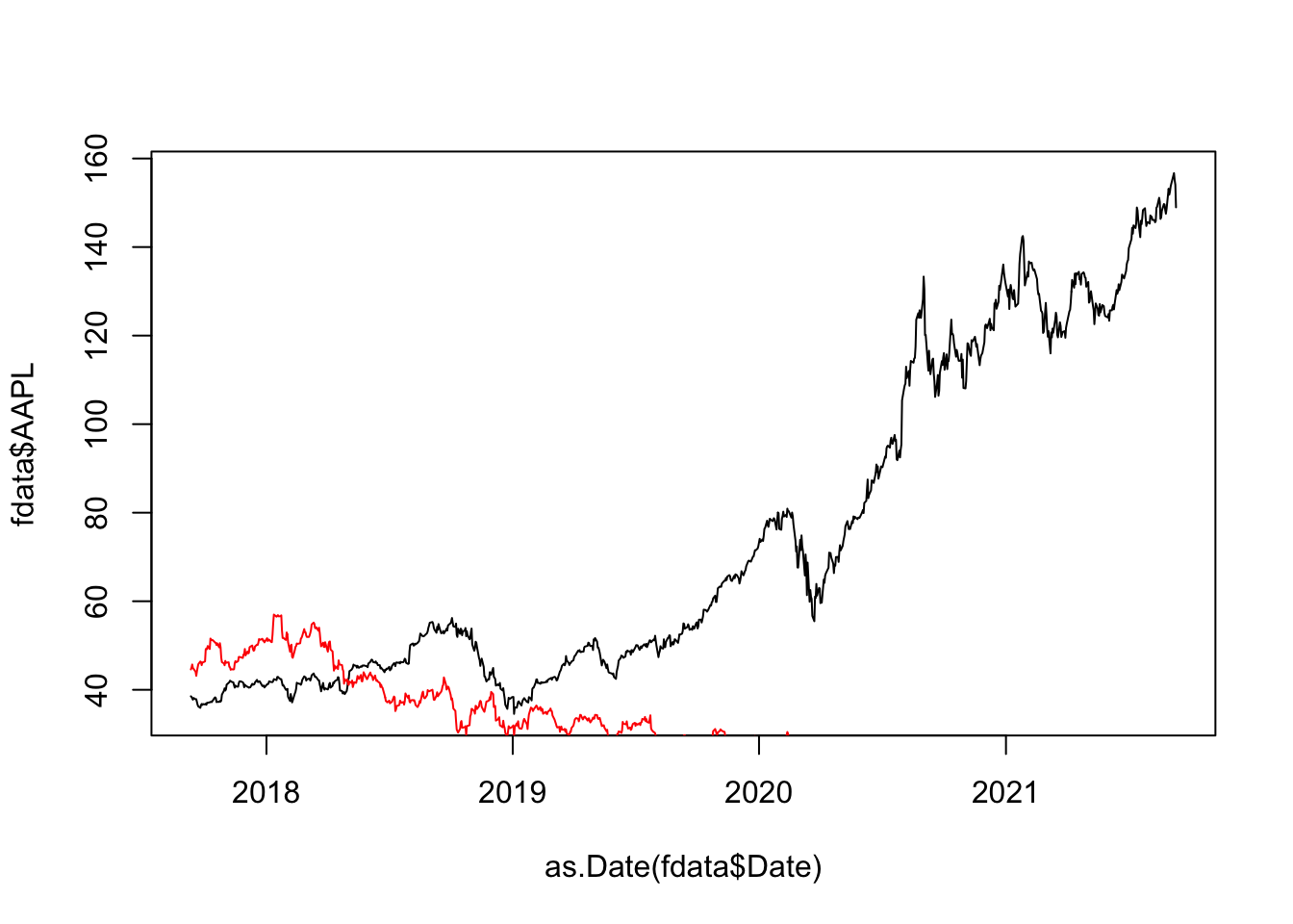

Note that the AAL time series is not visible because it is defined on a completely different range (check with summary). For this reason we have to change the range of the y axis by using the ylim argument of the plot function:

plot(as.Date(fdata$Date) , fdata$AAPL,
     type="l" , ylim = c(0,160))
#add a new time series here
lines(as.Date(fdata$Date) , fdata$AAL,
      col = "red")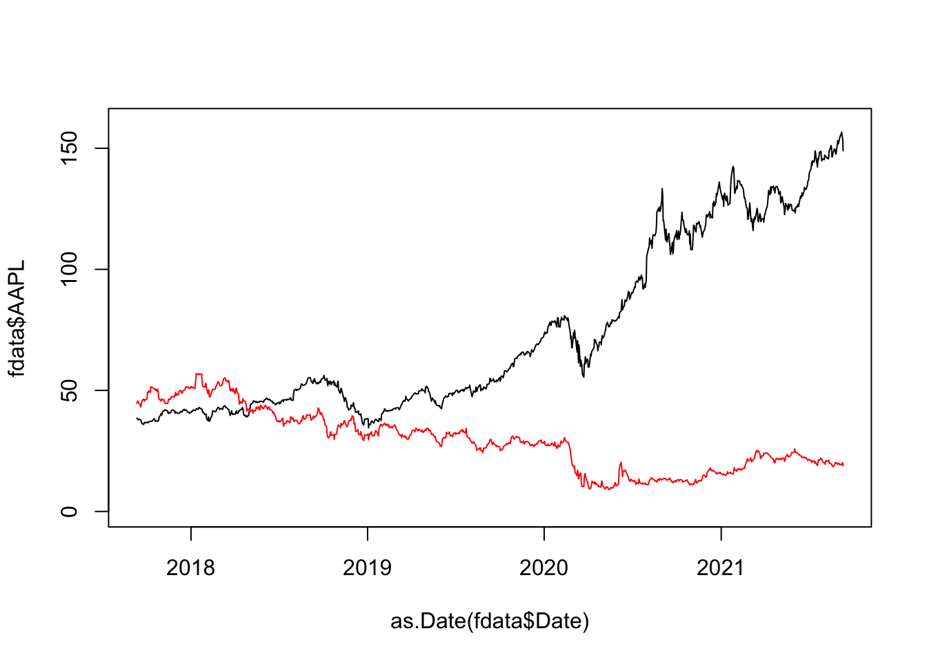

Finally, with the same approach it is possible to represent all together the 6 time series (in this case five of them look completely flat due to the very different range of values):

plot(as.Date(fdata$Date), fdata$AAPL,
     type="l" , ylim = c(0,max(fdata2)), 
     xlab="Financial dates", ylab="Prices",
     main="Time series plot")
lines(as.Date(fdata$Date) , fdata$GSAT,
      col = "red")
lines(as.Date(fdata$Date) , fdata$AMC,
      col = "green")
lines(as.Date(fdata$Date) , fdata$AAL,
      col = "orange")
lines(as.Date(fdata$Date) , fdata$F,
      col = "blue")
lines(as.Date(fdata$Date) , fdata$IXIC,
      col = "purple")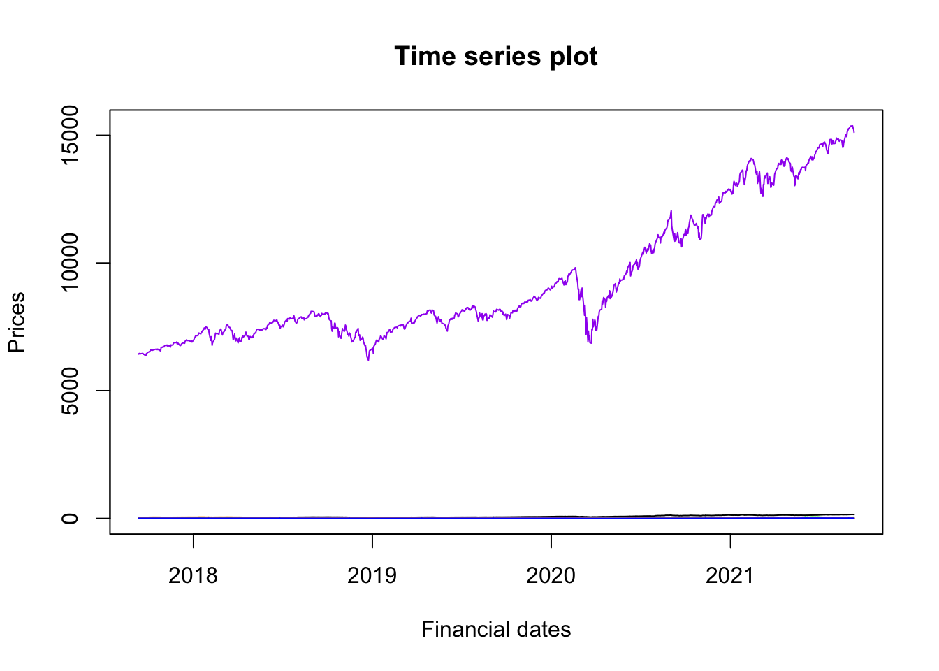

Note that the arguments xlab, ylab and main of the plot function are used to specify the x- and y-labels and the plot title, respectively.

You may be interested in adding a legend to the plot. This is the code you need (not requested for the exam!):

plot(as.Date(fdata$Date), fdata$AAPL,
     type="l" , ylim = c(0,max(fdata2)), 
     xlab="Financial dates", ylab="Prices",
     main="Time series plot")

lines(as.Date(fdata$Date) , fdata$GSAT,
      col = "red")
lines(as.Date(fdata$Date) , fdata$AMC,
      col = "green")
lines(as.Date(fdata$Date) , fdata$AAL,
      col = "orange")
lines(as.Date(fdata$Date) , fdata$F,
      col = "blue")
lines(as.Date(fdata$Date) , fdata$IXIC,
      col = "purple")
legend("topleft", 
       lty = rep(1,6), #line style 1=straight line
       col = c("black","red","green","orange","blue","purple"),
       legend = colnames(fdata)[2:ncol(fdata)],
       cex=0.5) #to reduce font size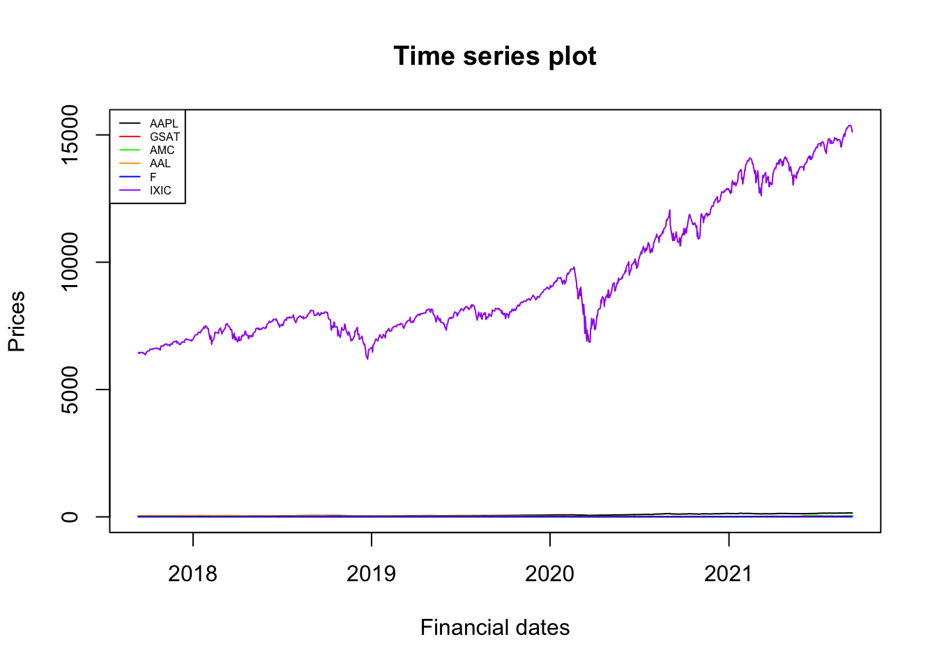

4.5 Compute returns

We start by computing log returns using the following definition: \[ r_t = \log\left(\frac{P_t}{P_{t-1}}\right) = log(P_t) - log(P_{t-1}) \] for $t=2, \ldots, n$.

In particular we will use the fact that log returns are given by the subsequent differences of log prices. The latter are compute by using the log functions, while differences are obtained by using the diff function. In order to discover how diff works, let’s consider a simple example with the first 5 prices of AAPL:

mini = fdata$AAPL[1:5]
mini

## [1] 38.53323 38.38054 38.09183 37.76495 38.14671

If we apply the function diff to the object (vector) mini we obtain a new vector

diff(mini)

## [1] -0.152699 -0.288704 -0.326877  0.381759

whose first value is the difference between the second price (38.380535) and the first one (38.533234). Similarly, the second difference is given by the differecen between the third price (38.091831) and the second one (38.533234). This is repeated day by day and returns the vector of differences whose lenght is given by $n-1$ (it’s not possible to compute the difference for the first day).

For computing log returns, we need first to compute the log prices and then to apply the diff functions to log prices:

diff(log(mini))

## [1] -0.00397066 -0.00755058 -0.00861832  0.01005806

Note that the order is important. Using log(diff(mini)) is NOT computing log-returns and is also given you error (because it is not possible to compute the log if the difference is negative)!

The first value of diff(log(mini)) is the first log return. To check it is possible to compute it manually:

log(mini[2]/mini[1])

## [1] -0.00397066

log(mini[2])-log(mini[1])

## [1] -0.00397066

The same approach can be used to compute the log returns for all the available days; they will be saved in a new object (vector) named AAPLlogret:

AAPLlogret = diff(log(fdata$AAPL)) 
length(AAPLlogret)

## [1] 1007

Once the log returns are available, the gross returns can be easily obtained by using the following formula: \[ \frac{P_t}{P_{t-1}} = \exp(r_t) \] The net returns instead are given by the following formula: \[ R_t = \frac{P_t}{P_{t-1}}-1 \]

Here below the code for computing the gross and net returns by using the log returns:

AAPLgrossret = exp(AAPLlogret)
AAPLnetret = AAPLgrossret - 1

It is possible to represent the three time series of returns by using the approach described in Section 4.4:

plot(AAPLgrossret, type="l", ylim=c(-0.5, 1.5),ylab="Returns")
lines(AAPLnetret, col="blue")
lines(AAPLlogret, col="red")
abline(h = 1, col="red") #add a constant horiziontal line at 1
abline(h = 0, col="green") #add a constant horiziontal line at 0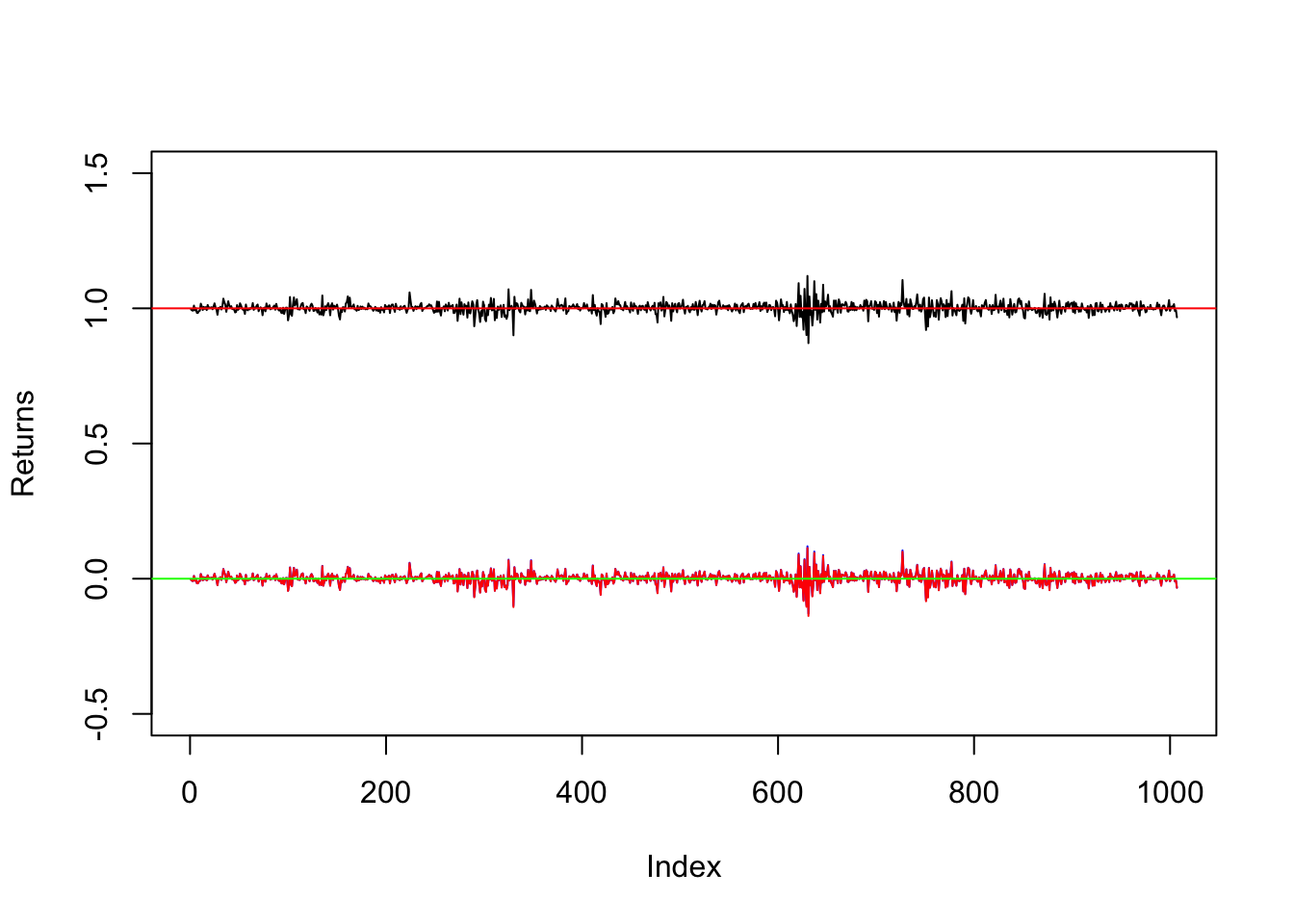

Note that the red series of log returns is covering almost entirely the blue series of net returns (this is given by the theoretical properties of returns, with $r_t\simeq R_t$ for small values of $R_t$).

The function abline is used to add a constant horizontal line for $y=1$ and $y=0$ which represent the reference value for the gross and net/log returns, respectively.

4.6 Exercises Lab 2

4.6.1 Exercise 1

Download from the e-learning (Lab2 folder) the 3 CSV files JNJ.csv, PFE.csv e NVS.csv (data source: https://finance.yahoo.com/). They refer to the price time series of the following assets for the period 03/10/2013 - 03/10/2018: Johnson & Johnson (JNJ), Pfizer Inc. (PFE) and Novartis AG (NVS). Each file contains the following variables (Currency in USD):

Date: date
Open: opening prices
High: highest price during the day
Low: lowest price during the day
Close: closing price adjusted for splits
Adj.Close: adjusted closing price adjusted for both dividends and splits
Volume: daily volume (how many shares are traded each day)

Import the data into R creating three different objects named JNJ, PFE and NVS. Pay attention to the field separator!

Have a look to the dataframes and check the structure (the quantitative variables should be classified as num or int).

Consider the Adj.Close prices. Compute for each asset some summary statistics (just one line of code). Which is the asset showing the highest variability?
By using the quantile function (see ?quantile) compute the median for the Adj.Close prices of JNJ. Comment the value.
We consider as extreme values the Adj.Close JNJ prices lower than 78$ or bigger than 140$ (hint: the condition OR in R is implemented through |).

How many extreme values do we observe?
What’s the mean value of these extreme values?

Plot in the same plot the three time series of Adj.Close prices. Comment the plot.
For each asset compute the percentage of prices (Adj.Close) greater than the mean. For which asset we observe the highest percentage?
Compute for JNJ the time series of log, gross and net returns. Save them in 3 different objects. Finally, represent the net and log returns in a single plot (dates are not required). Do you observe some differences?

4.6.2 Exercise 2

Import the data from the file worldbankdata.csv (see the Lab2 - files folder) which contains for 25 European countries information about the following variables: Population density (people per sq. km of land area) 2016, Electric power consumption (kWh per capita) 2014, Proportion of seats held by women in national parliaments (%) 2016, Mobile cellular subscriptions 2016, Rail lines (total route-km) 2014.

Extract all the data available for the 3rd country.
Extract all the data for the country whose name (in the Country variable) is Croatia. In this case you have to set a condition on the variable Country and to check when it is equal (use ==) to "Croatia".
Extract all the values for the variable pop_density. Which the country with the highest density?
Extract the Country and pop_density column. Which the country with the highest density?
Compute the median and the mean of the variable pop_density.