Chapter 5 Spatial Joins
A spatial join will likely be one of the most common types of overlay analyses you will employ in your analyses. In a spatial join the goal is to combine the attribute data from one geographic dataset (the join dataset) and append it to the geometry of another geographic dataset (the target dataset), based on the spatial relationship between the two datasets (figure 5.1. In a spatial join, the join dataset typically has 1 to 2 more dimensions that of the target features (recall that polygons are 2 dimensional, lines are 1 dimensional and points are 0 dimensional).
Usually the goal in a spatial join is to summarize or aggregate attribute information of either points that fall on/within the geometry of polygon or line features, or, to summarize the attribute information of lines that fall within polygons. In a transportation safety context, a good example would be to aggregate crash point data to the neighbourhood it occured within (point-in-polygon), or the number of crashes that occur on a road segment (points-on-lines). Another transportation example would be to aggregate the road network features by neighbourhoods (lines-in polygons).
For example in Figure 5.1 we have the crash point map where each crash has an ID. We also have a neighbourhood map with the names of neighbourhoods. We want to join the neighbourhood names to the point data, based on the co-location of the points and the neighbourhoods. We define the crash points dataset as the “target dataset.” The target dataset is the one where we want to preserve the existing geometry and attributes. We define the neighbourhood polygon dataset as the “join dataset.” THe join dataset contains the attribute information we want to join to the attribute table of the target dataset. In short, when we run a spatial join we preserve the geometry of the target dataset and add the attribute information of the join dataset.
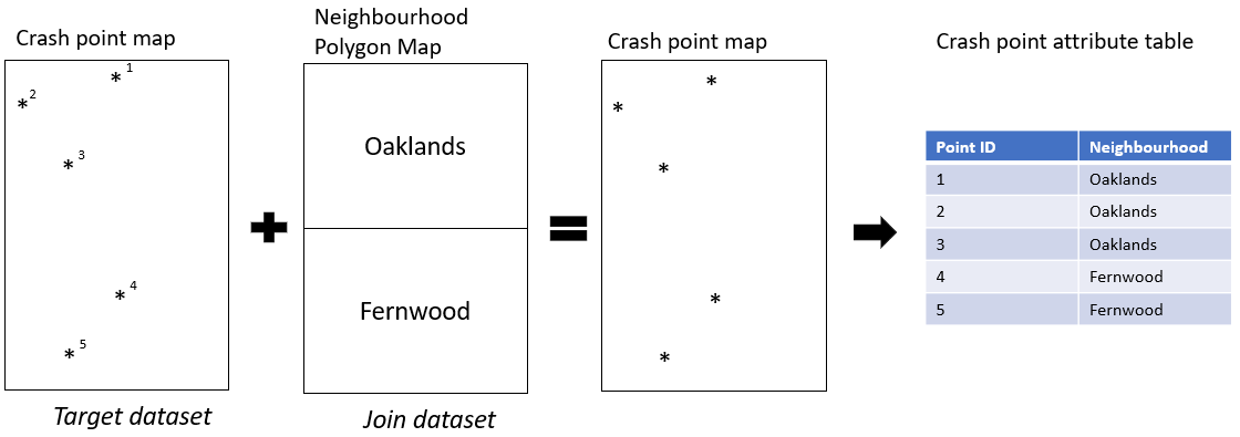
Figure 5.1: Diagram showing spatial join of polygons to points
ta.
In R we can use the st_join() function from the sf package to accomplish a spatial join. In this function the arguments that are input are st_join(x,y,join) where x refers to a target dataset (which needs to be an sf object), y refers to the join dataset. The default spatial relationship to use to define which feature attributes from the join dataset will be added to to which features from the target dataset is based on an intersection (i.e. st_intersects()). This can be modified to join attributes based on a different spatial relationship such as st_contains() or st_is_within_distance() among others. See the reference page for the full list.
Let’s go a through a few examples based on different purposes.
5.0.0.1 Points-in-polygon
In this example our end goal is to map the number of ICBC recorded bicycle crashes by dissemination area boundaries for the city of Vancouver. We will use the datasets we loaded earlier in the chapter:
vancouver_da_dep: Dissemination Area census geographies that include information on deprivation levels (see Attribute Join section above)icbc_crash_van: ICBC bicycle crash data for the City of Vancouver (see Buffer section above)
To enable counting of crashes within each dissemination area we are going to use a spatial join within a series of steps that will also draw upon what we learned about attribute joins and some data summary functionality from dplyr.
The first step is to join the DA level information to each point based on whether the point intersects with that polygon. Essentially, we want to take all of the DA level information and join it to each crash event based on the colocation of the crash and census data.
icbc_crash_van_join_da <- st_join(icbc_crash_van,vancouver_da_dep)
head(icbc_crash_van_join_da)
## Simple feature collection with 6 features and 49 fields
## Geometry type: POINT
## Dimension: XY
## Bounding box: xmin: 492170.9 ymin: 5458315 xmax: 494873.9 ymax: 5458438
## Projected CRS: NAD83 / UTM zone 10N
## # A tibble: 6 x 50
## `Crash Breakdown~ `Date Of Loss Ye~ `Crash Severity` `Cyclist Flag` `Day Of Week` `Derived Crash Cong~ `Intersection Cr~ `Month Of Year` `Motorcycle Fla~ `Municipality Nam~ `Parking Lot Fl~
## <chr> <dbl> <chr> <chr> <chr> <chr> <chr> <chr> <chr> <chr> <chr>
## 1 LOWER MAINLAND 2018 CASUALTY Yes SATURDAY SINGLE VEHICLE Yes MAY No VANCOUVER No
## 2 LOWER MAINLAND 2017 PROPERTY DAMAGE ~ Yes THURSDAY UNDETERMINED Yes MARCH No VANCOUVER No
## 3 LOWER MAINLAND 2015 CASUALTY Yes FRIDAY SINGLE VEHICLE Yes JUNE No VANCOUVER No
## 4 LOWER MAINLAND 2015 CASUALTY Yes WEDNESDAY SINGLE VEHICLE Yes JUNE No VANCOUVER No
## 5 LOWER MAINLAND 2016 CASUALTY Yes THURSDAY SINGLE VEHICLE Yes NOVEMBER No VANCOUVER No
## 6 LOWER MAINLAND 2019 PROPERTY DAMAGE ~ Yes WEDNESDAY SINGLE VEHICLE Yes JANUARY No VANCOUVER No
## # ... with 39 more variables: Pedestrian Flag <chr>, Region <chr>, Street Full Name (ifnull) <chr>, Time Category <chr>, Crash Breakdown <chr>, Cross Street Full Name <chr>,
## # Heavy Veh Flag <chr>, Mid Block Crash <chr>, Municipality Name <chr>, Municipality With Boundary <chr>, Road Location Description <chr>, Street Full Name <chr>, Crash Count <dbl>,
## # Number of Records <dbl>, geometry <POINT [m]>, uniqid <int>, Population <int>, Households <int>, GeoUID <chr>, Type <fct>, CD_UID <chr>, Shape Area <dbl>, Dwellings <int>, CSD_UID <chr>,
## # CT_UID <chr>, CMA_UID <chr>, Region Name <fct>, Area (sq km) <dbl>, v_CA16_2397 <dbl>, Province <chr>, Dissemination area (DA) Population <dbl>,
## # Ethno-cultural composition Quintiles <dbl>, Ethno-cultural composition Scores <dbl>, Situational vulnerability Quintiles <dbl>, Situational vulnerability Scores <dbl>,
## # Economic dependency Quintiles <dbl>, Economic dependency Scores <dbl>, Residential instability Quintiles <dbl>, Residential instability Scores <dbl>In the attribute table of our new object icbc_crash_van_join_da we can see that each point now has information for the dissemination area with which it is located (e.g. intersects with). A successful spatial join! But how do we go from here to map the number of crashes by dissemination area? The next step is to take our spatially joined data and use dplyr to group the data by the dissemination area unique identifier, add up the Crash Count variable for each row with the same unique id. Right now our data is still an sf point object. Now that the spatial join is done, we don’t need to keep the geometry associated with this feature so we can remove it using the st_drop_geometry() function. This will speed up the computation time for the functions performed on grouped data.
In the code chunk below we are grouping our data by the dissemination area unique id we just joined to our point data using the group_by() function and summing the Crash Count variable using the summarise() function.
no_icbc_crashes_by_da <-   icbc_crash_van_join_da %>%
  st_drop_geometry() %>%
  group_by(GeoUID) %>%
  summarise(total_crashes = sum(`Crash Count`))
The output is a table with one row for each dissemination area (unique GeoUID)
head(no_icbc_crashes_by_da)## # A tibble: 6 x 2
## GeoUID total_crashes
## <chr> <dbl>
## 1 59150310 1
## 2 59150311 1
## 3 59150313 4
## 4 59150329 3
## 5 59150330 1
## 6 59150332 1Now we have counts of crashes by the unique identifier of the dissemination area it occured in. Now we can simply join this table back to the polygon data using a left_join().
vancouver_da_dep_crashes <- left_join(vancouver_da_dep,no_icbc_crashes_by_da,by="GeoUID")


head(vancouver_da_dep_crashes)
## Simple feature collection with 6 features and 24 fields
## Geometry type: MULTIPOLYGON
## Dimension: XY
## Bounding box: xmin: 497754.1 ymin: 5458297 xmax: 498323.1 ymax: 5460083
## Projected CRS: NAD83 / UTM zone 10N
## Population Households GeoUID Type CD_UID Shape Area Dwellings CSD_UID CT_UID CMA_UID Region Name Area (sq km) v_CA16_2397 Province Dissemination area (DA) Population
## 1 632 254 59150307 DA 5915 0.29926 273 5915022 9330053.02 59933 Vancouver 0.29926 90965 British Columbia 669.4691
## 2 501 203 59150308 DA 5915 0.10956 223 5915022 9330053.02 59933 Vancouver 0.10956 93611 British Columbia 470.3942
## 3 745 269 59150309 DA 5915 0.11190 299 5915022 9330053.02 59933 Vancouver 0.11190 84736 British Columbia 728.7991
## 4 536 283 59150310 DA 5915 0.10940 310 5915022 9330053.02 59933 Vancouver 0.10940 45184 British Columbia 396.3275
## 5 532 181 59150311 DA 5915 0.08094 199 5915022 9330053.02 59933 Vancouver 0.08094 82517 British Columbia 623.7097
## 6 562 203 59150312 DA 5915 0.08706 211 5915022 9330053.02 59933 Vancouver 0.08706 74368 British Columbia 530.6063
## Ethno-cultural composition Quintiles Ethno-cultural composition Scores Situational vulnerability Quintiles Situational vulnerability Scores Economic dependency Quintiles
## 1 3 -0.2744621 2 -0.4505756 1
## 2 3 -0.2350062 1 -0.7415757 2
## 3 4 0.5496419 1 -0.6846734 2
## 4 4 0.8662144 5 0.3722661 2
## 5 4 0.6849209 2 -0.4435429 2
## 6 5 1.0570569 3 -0.2977577 1
## Economic dependency Scores Residential instability Quintiles Residential instability Scores total_crashes geometry
## 1 -0.9301352 4 0.1246316 NA MULTIPOLYGON (((498308 5459...
## 2 -0.6086799 2 -0.5748885 NA MULTIPOLYGON (((498301.6 54...
## 3 -0.6227231 3 -0.2030643 NA MULTIPOLYGON (((497939.5 54...
## 4 -0.4802208 5 1.9569124 1 MULTIPOLYGON (((498298.6 54...
## 5 -0.5483774 3 -0.4832458 1 MULTIPOLYGON (((498128.4 54...
## 6 -0.7775863 3 -0.1416693 NA MULTIPOLYGON (((498298.6 54...Our new column total_crashes has NA values for some polygons. This is because if a dissemination area did not have crashes occur within their boundaries they would not have been attribtued to a crash in our point dataset during the spatial join. The NA value actually then represents a 0. So let’s change the NA values to 0 using the replace_na() function from the tidyr package.
vancouver_da_dep_crashes <- vancouver_da_dep_crashes %>%
  mutate(total_crashes = replace_na(total_crashes,0))
Now let’s map the number of crashes from the new dataset vancouver_da_dep_crashes and overlay the original crash data icbc_crash_van
mapview(vancouver_da_dep_crashes,zcol = "total_crashes") + mapview(icbc_crash_van)5.0.0.2 Points-on-line
In a points-on-line spatial join we are applying the same concept as the previous example, but we instead want to join attribute data from line data to our point data. This type of operation is a bit trickier to implement because lines only 1-dimensions. So if a point does not fall exactly onto it’s geometry it is harder to join based on an intersection. There are a few ways around this as is the case with almost any kind of geoprocessing task. The simplest way would be to change spatial relationship from the default st_intersects to something like st_is_within_distance and specify a distance tolerance for considering a line to be attributed to a point. This is great if you are okay with a one-to-many spatial join where you create a new point object for every line segment within this distance. However, if we wanted to ensure a one-to-one join where you only join the attribute data from one line segment to one point - you will need to find a work around. One way to do this is to “snap” each point data to the nearest road segment, and then use the within st_join(x,y,join = st_is_within_distance, dist = tiny_value_like_1cm) to conduct the spatial join.
sf does not have a built in function for snapping points to nearest line segment but we can create one ourselves. Below is a function called st_snap_points() we define manually. It has 4 arguments, x for the point data, y for the line data, max_dist is the distance tolerance value, and namevar for specifying any uniqid from th original dataset. Feel free to ignore the details of the function below but make sure to run it before going through the rest of the section.
st_snap_points <- function(x, y, namevar, max_dist = 1000) {

  # this evaluates the length of the data
  if (inherits(x, "sf")) n = nrow(x)
  if (inherits(x, "sfc")) n = length(x)

  # this part:
  # 1. loops through every piece of data (every point)
  # 2. snaps a point to the nearest line geometries
  # 3. calculates the distance from point to line geometries
  # 4. retains only the shortest distances and generates a point at that intersection
  out = do.call("c",
                lapply(seq(n), function(i) {
                  nrst = st_nearest_points(st_geometry(x)[i], y)
                  nrst_len = st_length(nrst)
                  nrst_mn = which.min(nrst_len)
                  if (as.vector(nrst_len[nrst_mn]) > max_dist) return(st_geometry(x)[i])
                  return(st_cast(nrst[nrst_mn], "POINT")[2])
                })
  )

  # this part converts the data to a dataframe and adds a named column of your choice
  out_xy <- st_coordinates(out) %>% as.data.frame()
  out_xy <- out_xy %>%
    mutate({{namevar}} := x[[namevar]]) %>%
    st_as_sf(coords=c("X","Y"), crs=st_crs(x), remove=FALSE)

  return(out_xy)
}
Now that we have defined this function let’s try out another scenario. Similar to the section above, our end goal is to map the number of bicycle crashes (icbc_van_crash) that occur on the separated bicycle infrastructure network in Vancouver (bicycle_proj). The steps do so are as follows:
- Snap the crash locations to the nearest line segment based on a reasonable distance threshold using the
st_snap_pointsfunction - Perform a spatial join where we join the attributes of the nearest line segment to each point
- Aggregate the attribute data of the new spatially joined data by a unique identifier of the line segment
- Join the aggregated data back to the line segment data based on the unique identifier
Snap Points
Set a max distance of 20m to snap points. Outside of 20m then we don’t consider them occurring on an infrastructure segment and the position of the event will stay the same. This function may take a bit of time to run.
icbc_snp <- st_snap_points(x = icbc_crash_van,#crash van
                           y = bicycle_proj, #network infrasructure data
                           max_dist = 20,
                           namevar = "uniqid") #this only returns the geometry - doesn't preserve attributes

icbc_snp <-  left_join(icbc_snp,
                       icbc_crash_van %>%
                         st_drop_geometry(),
                       by = "uniqid")#return the attributes to the snapped locations


mapview(icbc_snp) + mapview(bicycle_proj)
Spatial Join
Now for each point let’s count the number of crashes that occur on that segment based on our 20m threshold. To do so we will join the unique id of the nearest road segment to the point data using st_join() and the st_within_distance() function. Since we already have snapped the points to the nearest road segment there is only one road segment assigned to each point and we specify a tiny distance to consider a spatial join.
icbc_snp_bicycle_inf <- st_join(icbc_snp,
                         bicycle_proj["osm_id"], #select only the column "osm_id"
                           join = st_is_within_distance, dist = 0.001) #for each point assign the LIXID that it falls on by indicating a very small distance tolerance (here it is 1mm)


icbc_snp_bicycle_inf %>%
  select(uniqid,`Crash Count`,osm_id) # look at the results
## Simple feature collection with 3405 features and 3 fields
## Geometry type: POINT
## Dimension: XY
## Bounding box: xmin: 484327.3 ymin: 5449979 xmax: 498329.2 ymax: 5462021
## Projected CRS: NAD83 / UTM zone 10N
## First 10 features:
## uniqid Crash Count osm_id geometry
## 1 42 1 <NA> POINT (492170.9 5458438)
## 2 43 1 368058222 POINT (492279.2 5458372)
## 3 45 1 <NA> POINT (492940 5458424)
## 4 46 1 368210443 POINT (494873.4 5458316)
## 5 47 1 368210443 POINT (494873.4 5458316)
## 6 48 1 368058222 POINT (492279.2 5458372)
## 7 51 1 748846437 POINT (490680.9 5458413)
## 8 52 1 <NA> POINT (492170.9 5458438)
## 9 56 1 827958314 POINT (491713.7 5458318)
## 10 57 1 540329767 POINT (490452.9 5458326)Note how only the points that were snapped to bicycle infrastructure locations have a uniqid assigned from the bicycle infrastructure data. The NA values indicate no lines were within a distance of 0.001 meters (i.e. equivalent to 20m since we snapped the points to the nearest segment based on a 20m threshold)
Spatial Aggregation
Now let’s count the number of points with same osm_id.
no_crashes_by_osm_id <- icbc_snp_bicycle_inf %>%
  group_by(osm_id) %>%
  summarise(n_crashes = sum(`Crash Count`)) %>%
  st_drop_geometry() # drop the geometry from this - we only need the uniqid for the bicycle infrastrucutre data and the counts
Attribute Join
Now we can join this data back to the bicycle infrastructure polyline data. Polylines without any crashes will be assigned an NA value because they don’t have a matching record in the join. We then simply replace the NA values with a 0 after the join using the replace_na() from the tidyr package.
bicycle_infra_crash_count <- left_join(bicycle_proj,no_crashes_by_osm_id , by = "osm_id") %>%
  mutate(n_crashes = replace_na(n_crashes,0))
Let’s map out the number of crashes by bicycle infrastructure and layer on the original point data and zoom into areas with collision events and see if the results make sense.
mapview(bicycle_infra_crash_count,zcol="n_crashes") + mapview(icbc_snp)5.0.0.3 Lines-in-polygon
Here let’s assume a scenario where the end goal is to calculate the length of separated bicycle infrastructure within each dissemination area in the City of Vancouver. Recall we created the following datasets from earlier in the chapter:
bicycle_proj: separated bicycle infrastructure polylines for the City of Vancouver in UTM Zone 10Nvancouver_da_dep: dissemination area boundaries for the City of Vancouver in UTM Zone 10N
The main problem is that as of now, the line segments for bicycle infrastructure do not line up with the boundary of disseminatin areas. This concept is illustrated in the left panel of Figure 5.1 where we have one polyline that crosses multiple boundaries. We need to cut the line segments where they intersect with the boundaries of dissemination areas such as in Figure 5.1 using st_intersection() so that we can then calculate the length of each individual segment using st_length().
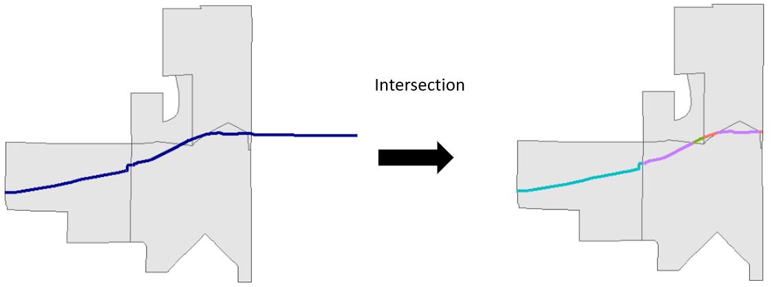
Figure 5.2: Intersection of a single polyline (blue) by polygons (grey)
From there we can sum the length of each line segment by the dissemination area’s unique identfier (GeoUID) in a few different ways, including a spatial join. Let’s try this out so we can see some of the problems that can arise with this type of data and operation.
First, let’s create the “cut” version of our bicycle infrastructure layer using st_intersection(). I am going to do this with subsets of original datasets that only contain the unique identifier as attribute data to make our data exploration a little cleaner.
## Warning: attribute variables are assumed to be spatially constant throughout all geometriesWe can then calculate the length of each line segment using a function called st_length().
bicycle_cut <- bicycle_cut %>%
  mutate(length_m = st_length(.))

bicycle_cut
## Simple feature collection with 1473 features and 3 fields
## Geometry type: GEOMETRY
## Dimension: XY
## Bounding box: xmin: 483720 ymin: 5449700 xmax: 498317.2 ymax: 5462376
## Projected CRS: NAD83 / UTM zone 10N
## First 10 features:
## osm_id GeoUID geometry length_m
## 35260598 35260598 59150307 LINESTRING (498105.5 545987... 157.80005 [m]
## 35260599 35260599 59150307 LINESTRING (497911 5459475,... 32.86117 [m]
## 36691655 36691655 59150307 LINESTRING (497911 5459475,... 163.86383 [m]
## 41840546 41840546 59150307 LINESTRING (498180.4 545988... 76.01887 [m]
## 75573893 75573893 59150307 LINESTRING (498226.7 545987... 44.49847 [m]
## 210638528 210638528 59150307 LINESTRING (498190.6 545997... 84.65905 [m]
## 210638530 210638530 59150307 LINESTRING (498235.3 545998... 46.27267 [m]
## 336365962 336365962 59150307 LINESTRING (497942.1 545946... 56.43094 [m]
## 340103260 340103260 59150307 LINESTRING (497944.5 545952... 86.09529 [m]
## 380516622 380516622 59150307 LINESTRING (498317.2 545999... 84.11612 [m]Notice how the intersection also attributed the GeoUID from the Dissemination Area boundary. We could then use that information to summarise the length of polylines within each GeoUID.
But let’s take a look at our data.
mapview(bicycle_cut) + mapview(vancouver_da_sub)Note how some bicycle infrastructure line segments follow the border of dissemination areas. One of the problems with trying to summarise transportation data within census polygons is that often the boundaries of census areas follow roads! So technically a given road belongs to more than one dissemination area. The intersection we performed above only assigned the attribute data from the neighbourhoods that intersected with a given road, a one-to-one spatial join. One way to deal with this would be to use the st_within_distance within st_join and create a polyline for each dissemination area that is within a certain distance of a line segment. This is called a one-to-many spatial join that will create multiple line segments for each dissemination where that spatial relationship is true. Let’s try it. If a line segment is within 5 metres of a dissemination area, join the attribute data from that dissemination area to the line segment. I chose 5 m to allow for some inaccuracy in the way the line data were digitized (e.g. a line segment may suppose to follow a boundary exactly but is actually a few metres off to one side etc.)
cut_join_da <- st_join(bicycle_cut, vancouver_da_sub,join = st_is_within_distance,dist=5)

cut_join_da
## Simple feature collection with 2585 features and 4 fields
## Geometry type: GEOMETRY
## Dimension: XY
## Bounding box: xmin: 483720 ymin: 5449700 xmax: 498317.2 ymax: 5462376
## Projected CRS: NAD83 / UTM zone 10N
## First 10 features:
## osm_id GeoUID.x length_m GeoUID.y geometry
## 35260598 35260598 59150307 157.80005 [m] 59150307 LINESTRING (498105.5 545987...
## 35260598.1 35260598 59150307 157.80005 [m] 59153215 LINESTRING (498105.5 545987...
## 35260599 35260599 59150307 32.86117 [m] 59150307 LINESTRING (497911 5459475,...
## 36691655 36691655 59150307 163.86383 [m] 59150307 LINESTRING (497911 5459475,...
## 41840546 41840546 59150307 76.01887 [m] 59150307 LINESTRING (498180.4 545988...
## 75573893 75573893 59150307 44.49847 [m] 59150307 LINESTRING (498226.7 545987...
## 210638528 210638528 59150307 84.65905 [m] 59150307 LINESTRING (498190.6 545997...
## 210638530 210638530 59150307 46.27267 [m] 59150307 LINESTRING (498235.3 545998...
## 336365962 336365962 59150307 56.43094 [m] 59150307 LINESTRING (497942.1 545946...
## 340103260 340103260 59150307 86.09529 [m] 59150307 LINESTRING (497944.5 545952...Note how the first two rows of our data have the same osm_id but different values for GeoUID.y. What this means is that for this particular line segment there are multiple dissemination areas that fullfill the spatial join criteria (is within 5 metres). Now we let’s summarise the length_m column by the GeoUID.y column.
length_by_da <- cut_join_da %>%
  st_drop_geometry() %>%
  group_by(GeoUID.y) %>%
  summarise(total_length_km = sum(as.numeric(length_m))/1000)

head(length_by_da)
## # A tibble: 6 x 2
## GeoUID.y total_length_km
## <chr> <dbl>
## 1 59150307 1.34
## 2 59150309 0.218
## 3 59150312 0.0560
## 4 59150313 0.0939
## 5 59150328 0.171
## 6 59150329 1.30Now let’s join this back to our dissemination area boundaries, replace the NAs with 0s and map the results!
vancouver_da_sub <- left_join(vancouver_da_sub,length_by_da , by = c("GeoUID"="GeoUID.y")) %>%
  mutate(total_length_km = replace_na(total_length_km,0))

vancouver_da_sub
## Simple feature collection with 993 features and 2 fields
## Geometry type: MULTIPOLYGON
## Dimension: XY
## Bounding box: xmin: 483690.9 ymin: 5449535 xmax: 498329.2 ymax: 5462381
## Projected CRS: NAD83 / UTM zone 10N
## First 10 features:
## GeoUID total_length_km geometry
## 1 59150307 1.33568195 MULTIPOLYGON (((498308 5459...
## 2 59150308 0.00000000 MULTIPOLYGON (((498301.6 54...
## 3 59150309 0.21754280 MULTIPOLYGON (((497939.5 54...
## 4 59150310 0.00000000 MULTIPOLYGON (((498298.6 54...
## 5 59150311 0.00000000 MULTIPOLYGON (((498128.4 54...
## 6 59150312 0.05595795 MULTIPOLYGON (((498298.6 54...
## 7 59150313 0.09386538 MULTIPOLYGON (((498259 5458...
## 8 59150328 0.17094843 MULTIPOLYGON (((498102 5458...
## 9 59150329 1.29789720 MULTIPOLYGON (((497801.1 54...
## 10 59150330 0.00000000 MULTIPOLYGON (((497312 5458...mapview(vancouver_da_sub,zcol = "total_length_km") + mapview(bicycle_sub)We could also map the density instead:
vancouver_da_sub <- vancouver_da_sub %>%
  mutate(total_area_km2 = as.numeric(st_area(.)/1000/1000),
         total_bike_dens = total_length_km/ total_area_km2
         )

mapview(vancouver_da_sub,zcol = "total_bike_dens")  + mapview(bicycle_sub)