Chapter 4 GIS Analysis Toolkit
This chapter requires the following packages:
library(sf)
library(readr)
library(readxl)
library(tidyr)
library(cancensus)
library(osmdata)
library(mapview)
library(dplyr)
The previous chapter was dedicated to getting the baseline skills necessary to load spatial data into R and understand the different data structures. In this section we are going to go over the basic geoprocessing operations that are commonly encountered in applied research with spatial data. Geoprocessing is a commonly used term for describing a suite of tools and operations that manipulate an existing spatial dataset to create new or augmented versions of the original data.
4.1 Attribute Queries
One of the most basic spatial data operations is to create subsets based on the values of an attribute (i.e a column). Let’s retrieve Metro Vancouver data using the cancensus package that was introduced in the previous chapter, and examine the attributes associated with each dissemination area. Note that the ID for Metro Vancouver is 5915. Feel free to augment the code below to retrieve a different subset of Canadian census data.
find_census_vectors("Median total income",type = "total", dataset = "CA16",query_type = "semantic")#options(cancensus.api_key = "your_api_key") # uncomment and input your API Key here to enable retrieval of data from Statistics Canada## # A tibble: 9 x 4
## vector type label details
## <chr> <fct> <chr> <chr>
## 1 v_CA16_2~ Total Median total income in 2015 among recipients ($) Income; Individuals; Total - Income statistics in 2015 for the population aged 15 years and over in private house~
## 2 v_CA16_2~ Total Median total income of households in 2015 ($) Income; Households; Total - Income statistics in 2015 for private households by household size - Median total inc~
## 3 v_CA16_2~ Total Median total income of one-person households in 2015 ($) Income; Households; Total - Income statistics in 2015 for one-person private households - Median total income of ~
## 4 v_CA16_2~ Total Median total income of two-or-more-person households in 20~ Income; Households; Total - Income statistics in 2015 for two-or-more-person private households - Median total in~
## 5 v_CA16_2~ Total Median total income of economic families in 2015 ($) Income; Families; Total - Income statistics in 2015 for economic families in private households - Median total in~
## 6 v_CA16_2~ Total Median total income of couple economic families without ch~ Income; Families; Total - Income statistics in 2015 for couple economic families without children or other relati~
## 7 v_CA16_2~ Total Median total income of couple economic families with child~ Income; Families; Total - Income statistics in 2015 for couple economic families with children in private househo~
## 8 v_CA16_2~ Total Median total income of lone-parent economic families in 20~ Income; Families; Total - Income statistics in 2015 for lone-parent economic families in private households - Med~
## 9 v_CA16_2~ Total Median total income in 2015 for persons aged 15 years and ~ Income; Families; Total - Income statistics in 2015 for persons aged 15 years and over not in economic families i~mv_census <- get_census(dataset='CA16', #specify the census of interest
regions=list(CSD="5915"),#specify the region of interest
vectors=c("v_CA16_2397"), # specify the attribute data of interest
labels = "short",# here we specify short variabhle names, otherwise they get very long
level='DA', #specify the census geography
geo_format = "sf", #specify the geographic data format as output
quiet = TRUE #turn off download progress messages (set to FALSE to see messages)
)
mv_census## Simple feature collection with 3450 features and 13 fields
## Geometry type: MULTIPOLYGON
## Dimension: XY
## Bounding box: xmin: -123.4319 ymin: 49.00192 xmax: -122.4086 ymax: 49.57428
## Geodetic CRS: WGS 84
## First 10 features:
## Population Households GeoUID Type CD_UID Shape Area Dwellings CSD_UID CT_UID CMA_UID Region Name Area (sq km) v_CA16_2397 geometry
## 1 368 159 59150004 DA 5915 0.85230 172 5915055 9330133.01 59933 West Vancouver 0.85230 94592 MULTIPOLYGON (((-123.2421 4...
## 2 503 205 59150005 DA 5915 0.16598 221 5915055 9330133.01 59933 West Vancouver 0.16598 102997 MULTIPOLYGON (((-123.2789 4...
## 3 432 196 59150006 DA 5915 0.15593 200 5915055 9330133.01 59933 West Vancouver 0.15593 85504 MULTIPOLYGON (((-123.2773 4...
## 4 546 212 59150007 DA 5915 0.71085 221 5915055 9330133.01 59933 West Vancouver 0.71085 133803 MULTIPOLYGON (((-123.289 49...
## 5 596 224 59150008 DA 5915 0.65167 247 5915055 9330133.01 59933 West Vancouver 0.65167 167936 MULTIPOLYGON (((-123.2815 4...
## 6 399 136 59150009 DA 5915 0.56986 143 5915055 9330133.01 59933 West Vancouver 0.56986 146432 MULTIPOLYGON (((-123.2797 4...
## 7 831 298 59150010 DA 5915 0.80527 314 5915055 9330133.01 59933 West Vancouver 0.80527 144725 MULTIPOLYGON (((-123.2766 4...
## 8 512 173 59150012 DA 5915 0.44894 182 5915055 9330133.02 59933 West Vancouver 0.44894 129792 MULTIPOLYGON (((-123.2429 4...
## 9 360 118 59150013 DA 5915 0.27287 122 5915055 9330133.02 59933 West Vancouver 0.27287 163328 MULTIPOLYGON (((-123.2429 4...
## 10 1070 413 59150014 DA 5915 32.12439 455 5915055 9330133.02 59933 West Vancouver 32.12439 123136 MULTIPOLYGON (((-123.195 49...Notice how our census data has attributes that describe geographical regions we are interested in via the column Region Name. While there are several ways to subset rows of data (spatial or otherwise) based on the values of columns, the filter() function from the dplyr package integrates nicely with sf objects, is intuitive and easy to implement. In the filter function we can construct a boolean expression (a statement that evaluates to either TRUE or FALSE) to determine which rows (which with sf objects, correspond to a spatial feature) we want to keep in our new dataset. Example functions and operators include:
==(is equal to)>(greater than)<(less than)is.na()(is equal to NA[ no value])
We can combine these functions using operators such as
&(and, to combine)|(or)!(does not equal)
Let’s try an attribute query that will isolate (or filter) the dissemination areas that are within the City of Vancouver and has a median household income > $175,000.
cov_high_income <- mv_census %>%
  filter(`Region Name`=="Vancouver" & v_CA16_2397 >175000)
In the above code we are stating that we want to create a new spatial dataset called cov_wealthy. THis new object is based on the original dataset mv_census where, using the filter() function, we only keep the rows (corresponding to a polygon) where the Region Name column value is equal to the string "Vancouver" AND the column describing the median household income v_CA16_2397 is greater than $175,000. Let’s see if this worked by quickly mapping both the original data and the new data using mapview(). Click on the red polygons and check to see if the value for v_CA16_2397 is greater than 175000.
mapview(mv_census) + mapview(cov_high_income,col.regions = "red")We can see that this attribute query has worked perfectly and that the layer coloured in red only contains dissemination areas within the City of Vancouver and where the median household income is greater than $175,000.
Now let’s do a slightly more complex attribute query using data retrieved from OpenStreetMaps using the osmdata package where we only want separated bicycle infrastructure data (E.g. lines representing the location of separated infrastructure). First let’s load data for the city
van_bb <- getbb("Vancouver BC")

streets <- van_bb %>%
  opq()%>%
  add_osm_feature(key = "highway") %>%
  osmdata_sf()

streets_sf <- streets$osm_lines
In the osm data there are several attributes (columns) that could be used to designate separated bicycling infrastructure including the “highway” column and the “bicycle” column. Here we construct a query that will select lines based on the different values that could be plausibly be used to describe separated bicycling infrastructure. In plain engligh this looks like.
Select the features where the following is TRUE:
highwayequals “cycleway” ORhighwayequals “path” &bicycleequals “yes” ORhighwayequals “path” &bicycleequals “designated” ORhighwayequals “footway” &bicycleequals “yes” ORhighwayequals “footway” &bicycleequals “designated”
bicycle <- streets_sf %>%
  filter(highway=="cycleway" | (highway=="path"&bicycle=="yes") | (highway=="path"&bicycle=="designated") | (highway=="footway"&bicycle=="yes") | (highway=="footway"&bicycle=="designated"))

 mapview(streets_sf) + mapview(bicycle,color = "red")
In the above map we can see our selection highlighted in red.
4.2 Spatial Queries
What happens if we wanted to isolate spatial data based on the location, but the data don’t have existing attributes that are associated with that location? For example, what if our census data did not have the Region Name column? One way we could solve this problem would be to find another spatial dataset that represents the location of interest, and perform what is called a spatial query. Spatial queries refer to creating new data or subsets of data based purely on the location of different features, in relation to another dataset. For example, if we wanted to select all the crashes within a certain distance of specific infrastructure types, we’d need to perform a spatial query. More formally, spatial queries are typically based on either topological spatial relationships or distance relationships. Topological relationships describe the relationship in terms of whether any two spatial data a and b intersects, touches, contains among others. While distance relationships are about how far away certain objects are from each other. Let’s get the flavour for a spatial query by going through a few examples.
First, let’s answer the first question I posed in the above paragraph. How would we isolate the Dissmimination Areas within the City of Vancouver, if our dataset did not have an existing attribute that describes which region the DA fell in? We will need another spatial dataset which represents the boundary of the City of Vancouver. Such a shapefile was included in the course data package in Chapter 1.
van_boundary <- read_sf("D:/Github/crash-course-gis-r/data/CoV_boundary.shp") # use the file location of where you have stored your data

mapview(mv_census) + mapview(van_boundary,col.regions = "red")
We can see from our map above that we want to keep those DAs that are within the red polygon (the City of Vancouver boundary). We can use functions from sf to evaluate the topological spatial relationships between these two datasets (See https://r-spatial.github.io/sf/reference/geos_binary_pred.html for a full list of operations). We are going to use the function st_interscts() to evaluate which polygons from the mv_census dataset intersect with the spatial features of the van_boundary dataset. First let’s just run the function setting the argument “sparse” = FALSE and see what the output is. We are setting the arugment sparse to false for teaching purposes, but I encourage you to read (Chapter 4)[https://geocompr.robinlovelace.net/spatial-operations.html#introduction-1] of Geocomputation with R for a greater background on the technical details.
st_intersects(mv_census,van_boundary,sparse = FALSE)## Error in st_geos_binop("intersects", x, y, sparse = sparse, prepared = prepared, : st_crs(x) == st_crs(y) is not TRUEShoot! We get an error message indicating that our two datasets are in two different coordinate systems! This is an important lesson to learn. In order to perform any kind of spatial operation involving more than one dataset, we need to ensure they are both in the same coordinate system.
Let’s troubleshoot this. First let’s check the CRS information of each dataset and compare.
st_crs(mv_census)#check CRS## Coordinate Reference System:
## User input: 4326
## wkt:
## GEOGCS["WGS 84",
## DATUM["WGS_1984",
## SPHEROID["WGS 84",6378137,298.257223563,
## AUTHORITY["EPSG","7030"]],
## AUTHORITY["EPSG","6326"]],
## PRIMEM["Greenwich",0,
## AUTHORITY["EPSG","8901"]],
## UNIT["degree",0.0174532925199433,
## AUTHORITY["EPSG","9122"]],
## AXIS["Latitude",NORTH],
## AXIS["Longitude",EAST],
## AUTHORITY["EPSG","4326"]]st_crs(van_boundary)#check CRS## Coordinate Reference System:
## User input: NAD83 / UTM zone 10N
## wkt:
## PROJCRS["NAD83 / UTM zone 10N",
## BASEGEOGCRS["NAD83",
## DATUM["North American Datum 1983",
## ELLIPSOID["GRS 1980",6378137,298.257222101,
## LENGTHUNIT["metre",1]]],
## PRIMEM["Greenwich",0,
## ANGLEUNIT["degree",0.0174532925199433]],
## ID["EPSG",4269]],
## CONVERSION["UTM zone 10N",
## METHOD["Transverse Mercator",
## ID["EPSG",9807]],
## PARAMETER["Latitude of natural origin",0,
## ANGLEUNIT["Degree",0.0174532925199433],
## ID["EPSG",8801]],
## PARAMETER["Longitude of natural origin",-123,
## ANGLEUNIT["Degree",0.0174532925199433],
## ID["EPSG",8802]],
## PARAMETER["Scale factor at natural origin",0.9996,
## SCALEUNIT["unity",1],
## ID["EPSG",8805]],
## PARAMETER["False easting",500000,
## LENGTHUNIT["metre",1],
## ID["EPSG",8806]],
## PARAMETER["False northing",0,
## LENGTHUNIT["metre",1],
## ID["EPSG",8807]]],
## CS[Cartesian,2],
## AXIS["(E)",east,
## ORDER[1],
## LENGTHUNIT["metre",1]],
## AXIS["(N)",north,
## ORDER[2],
## LENGTHUNIT["metre",1]],
## ID["EPSG",26910]]Based on the CRS information above, we see that the mv_census dataset is “unprojected” and is in WGS1984, while van_boundary is in the projected coordinated system of NAD83/UTM Zone 10N. Since we need our data to be projected, let’s tranform the mv_census object to be in the same projection as van_boundary.
crs_to_use <- st_crs(van_boundary) # store crs information from the van_boundary dataset
crs_epsg <- crs_to_use$epsg # store the epsg code from the van_boundary dataset

mv_census_proj <- st_transform(mv_census,crs=crs_epsg)
Now let’s check to see if they are both in the same coordinate system
st_crs(van_boundary)==st_crs(mv_census_proj)## [1] TRUEGreat! We are rolling now. Let’s try the spatial operation of st_intersects() again, and see what the output is
st_intersects_output <- st_intersects(mv_census_proj,van_boundary,sparse = FALSE)

head(st_intersects_output)
## [,1]
## [1,] FALSE
## [2,] FALSE
## [3,] FALSE
## [4,] FALSE
## [5,] FALSE
## [6,] FALSEWhen we set the argument “sparse” = FALSE, what is returned is matrix where each row corresponds to a spatial feature within the mv_census_proj object and if the value is TRUE than it means that the feature intersects with the van_boundary geometry and if FALSE than it means it does not. We can combine this output with the the filter() function to return only the polygons that intersect with the van_boundary polygon.
census_intersects <- filter(mv_census_proj,st_intersects(x = mv_census_proj, y = van_boundary, sparse = FALSE))

mapview(van_boundary,col.region = "red") + mapview(census_intersects)
Another important lesson to learn here! It looks like our spatial query returned the dissemination areas just on the borders of the van_boundary file. This is a common occurrence in GIS analysis where boundaries from different data sources don’t exactly line up. You can see that the borders of the red polygon representing the City of Vancouver boundaries don’t line up with borders of our dissemination areas, causing us to select polygons that intersect with the Vancouver boundary layer, but are technically in Richmond, Burnaby and UBC. This is why it is important to map out your geoprocessing to do a spot check on whether what you wanted to do, actually occurred.
Now let’s brainstorm on how we can fix this problem. Short of manually fixing the boundaries to ensure that they line up with the dissemination area boundaries, we need to get a bit creative. I’m going to introduce you to the concept of a centroid, something that can be quite handy in situations like these. A centroid in GIS speak, is the “average” coordinate within a polygon, that is a single point (x,y location) that is representative of the location of a polygon.
mv_centroids <- st_centroid(mv_census_proj)

mapview(van_boundary,col.regions="red") + mapview(mv_census_proj) + mapview(mv_centroids,col.regions="black")
Make sure to explore this map by zooming in and clicking on the points and the polygons they fall on. See if you can find any polygons where the centroid doesn’t fall within the boundaries of its polygon. Zoom into areas around the border of the red polygon and see if any of the centroid fall within it.
When we are working with two polygon datasets whose boundaries don’t align in the way we want, often using the centroids to represent a polygon location can be a good solution to this problem. Instead of selecting disseminiation area polygons whose boundaries intersect with the Vancouver boundary, let’s select the dissmeination area polygons whose centroid intersects with the Vancouver boundary layer. We can do this by combining filter(), st_intersect() and st_centroid().
census_intersects_cntrd <- filter(mv_census_proj,st_intersects(x = st_centroid(mv_census_proj), y = van_boundary, sparse = FALSE))

mapview(van_boundary,col.region = "red") + mapview(census_intersects_cntrd)
There we have it. Explore the output in the map to ensure that we have selected the correct polygons.
This section was designed to give you some intuition as to how to perform a spatial query. There are lots of different ways of conducting spatial queries to produce the spatial dataset you need. Check out a (full list of functions)[https://r-spatial.github.io/sf/reference/geos_binary_pred.html] to give you an idea of what other topological and distance relationships you can query using sf.
4.3 Attribute Joins
Often data are provided in tabular format that are associated with a certain geographic location such as census geographies (census tracts, dissemination areas etc.) or neighbourhoods, or other geographic identifiers. For example in your downloaded data there is an excel spread sheet called bc_scores_quintiles_EN.xlsx which is originally from Statistics Canada that provides a score for different dimensions deprivation for each dissemination area in the province of British Columbia. In the figure below the column that refers to a unique identifier for each dissemination area in the province is named “PRCDDA.”
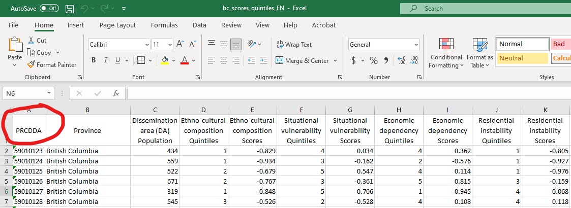
Figure 4.1: Tabular data with unique geographic identifier
That same variable is available within the census data we have previously retrieved in the chapter. As can be seen in the figure below, within the census data retrieved using cancensus the dissemination area unique identifier is named “GeoUID.” With this knowledge in mind we can join the spread sheet data that lacks any geometry to our sf census data using this unique identifier.
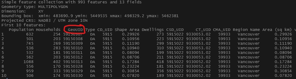
Figure 4.2: Geographic data with unique geographic identifier
First we need to use the function read_xlsx() from the readxl package to load in the .xlsx excel spreadsheet data.
deprivation_da <- read_xlsx("D:/Github/crash-course-gis-r/data/bc_scores_quintiles_EN.xlsx",sheet = 1)Then we use the function left_join() from the dplyrpackage. The left_join() function takes two datasets and returns all the rows from x and only the rows from y where there is a matching value.
](images/left_join.png)
Figure 4.3: Excample of left join operation for two datasets.source
While there are many kind of ways to join tables together based on common attributes (see here), here we are interested in ensuring that we keep all of the geographic data and only the data on deprivation for the dissemination areas we are interested in.
In this function we make sure to input our geographic sf object first to indicate that is the dataset for which we wish to keep all the records (e.g. circle A in the above figure), and the a-spatial tabular data second to indicate that is the data we wish to join matching records. We can indicate that our unique identifier we use to match the records have different names in each dataset. The other alternative is to rename one of the variables to match the other, but this works also.
vancouver_da_dep <- left_join(census_intersects_cntrd,deprivation_da, by = c("GeoUID"="PRCDDA"))Let’s take a look at the data and then map it out to ensure it worked.
vancouver_da_dep## Simple feature collection with 993 features and 23 fields
## Geometry type: MULTIPOLYGON
## Dimension: XY
## Bounding box: xmin: 483690.9 ymin: 5449535 xmax: 498329.2 ymax: 5462381
## Projected CRS: NAD83 / UTM zone 10N
## First 10 features:
## Population Households GeoUID Type CD_UID Shape Area Dwellings CSD_UID CT_UID CMA_UID Region Name Area (sq km) v_CA16_2397 Province Dissemination area (DA) Population
## 1 632 254 59150307 DA 5915 0.29926 273 5915022 9330053.02 59933 Vancouver 0.29926 90965 British Columbia 669.4691
## 2 501 203 59150308 DA 5915 0.10956 223 5915022 9330053.02 59933 Vancouver 0.10956 93611 British Columbia 470.3942
## 3 745 269 59150309 DA 5915 0.11190 299 5915022 9330053.02 59933 Vancouver 0.11190 84736 British Columbia 728.7991
## 4 536 283 59150310 DA 5915 0.10940 310 5915022 9330053.02 59933 Vancouver 0.10940 45184 British Columbia 396.3275
## 5 532 181 59150311 DA 5915 0.08094 199 5915022 9330053.02 59933 Vancouver 0.08094 82517 British Columbia 623.7097
## 6 562 203 59150312 DA 5915 0.08706 211 5915022 9330053.02 59933 Vancouver 0.08706 74368 British Columbia 530.6063
## 7 1088 402 59150313 DA 5915 0.17284 418 5915022 9330052.02 59933 Vancouver 0.17284 61184 British Columbia 954.5501
## 8 556 170 59150328 DA 5915 0.23224 181 5915022 9330052.02 59933 Vancouver 0.23224 80896 British Columbia 558.0631
## 9 959 333 59150329 DA 5915 0.30854 356 5915022 9330052.02 59933 Vancouver 0.30854 66688 British Columbia 891.8479
## 10 506 174 59150330 DA 5915 0.07820 189 5915022 9330052.02 59933 Vancouver 0.07820 82176 British Columbia 460.2466
## Ethno-cultural composition Quintiles Ethno-cultural composition Scores Situational vulnerability Quintiles Situational vulnerability Scores Economic dependency Quintiles
## 1 3 -0.2744621 2 -0.4505756 1
## 2 3 -0.2350062 1 -0.7415757 2
## 3 4 0.5496419 1 -0.6846734 2
## 4 4 0.8662144 5 0.3722661 2
## 5 4 0.6849209 2 -0.4435429 2
## 6 5 1.0570569 3 -0.2977577 1
## 7 4 0.5790914 5 0.6069958 3
## 8 5 1.4650933 3 -0.2751484 1
## 9 5 2.4115451 4 0.0428343 4
## 10 5 0.9880264 3 -0.2410908 1
## Economic dependency Scores Residential instability Quintiles Residential instability Scores geometry
## 1 -0.9301352 4 0.1246316 MULTIPOLYGON (((498308 5459...
## 2 -0.6086799 2 -0.5748885 MULTIPOLYGON (((498301.6 54...
## 3 -0.6227231 3 -0.2030643 MULTIPOLYGON (((497939.5 54...
## 4 -0.4802208 5 1.9569124 MULTIPOLYGON (((498298.6 54...
## 5 -0.5483774 3 -0.4832458 MULTIPOLYGON (((498128.4 54...
## 6 -0.7775863 3 -0.1416693 MULTIPOLYGON (((498298.6 54...
## 7 -0.0186630 4 0.2009225 MULTIPOLYGON (((498259 5458...
## 8 -1.4517890 3 -0.2034135 MULTIPOLYGON (((498102 5458...
## 9 0.1864334 3 -0.3812451 MULTIPOLYGON (((497801.1 54...
## 10 -0.7402528 2 -0.6010522 MULTIPOLYGON (((497312 5458...mapview(vancouver_da_dep, zcol = "Residential instability Scores")4.4 Buffers
Buffers are a geometric operation which creates a polygon based on a specified distance around individual spatial features. Buffers can be constructed around points, line and polygons.
](images/GIS_Buffer.png)
Figure 4.4: Diagram showing a buffer (green) of a point, line and polygon feature (red).Source
Let’s illustrate with a few examples.
First let’s load some data. Recall the code from last chapter to convert the .csv data on crash events to a spatial object in R. Below we repeat that code.
icbc_crash <- read_csv("D:/Github/crash-course-gis-r/data/ICBC_cyclist_crashes.csv") %>%# use the file location of where you have stored your data
    filter(!is.na(Latitude)) %>% # remove the recrods which have missing values
  st_as_sf(.,coords = c("Longitude","Latitude"),crs = 4326) %>%
  mutate(uniqid = row_number()) #assign unique identifier to each crash record
##
## -- Column specification ------------------------------------------------------------------------------------------------------------------------------------------------------------------------
## cols(
## .default = col_character(),
## `Date Of Loss Year` = col_double(),
## `Crash Count` = col_double(),
## Latitude = col_double(),
## Longitude = col_double(),
## `Number of Records` = col_double()
## )
## i Use `spec()` for the full column specifications.Now on your own select the crashes that occur within the City of Vancouver and assign it to a new spatial object called icbc_crash_van.
HINT you can do either an attribute query or a spatial query and you will need to convert the layer to a projected coordinate system.
The output should look like this:
mapview(icbc_crash_van)Buffers can be created using the function st_buffer() from the sf package and inputting the sf object that you wish to create buffers around, and the size of the buffer in a unit of length (e.g. metres). Check the units of your map projection to ensure you know what numbers to input for distance. Here let’s create a 200m buffer around each crash event in our dataset.
st_crs(icbc_crash_van)$units # my map projection uses metres as a unit - ## [1] "m"crash_buffer_icbc <- st_buffer(icbc_crash_van,dist = 150)
crash_buffer_icbc## Simple feature collection with 3373 features and 26 fields
## Geometry type: POLYGON
## Dimension: XY
## Bounding box: xmin: 484177.4 ymin: 5449829 xmax: 498479.2 ymax: 5462176
## Projected CRS: NAD83 / UTM zone 10N
## # A tibble: 3,373 x 27
## `Crash Breakdown~ `Date Of Loss Ye~ `Crash Severity` `Cyclist Flag` `Day Of Week` `Derived Crash Con~ `Intersection Cr~ `Month Of Year` `Motorcycle Fla~ `Municipality Nam~ `Parking Lot Fl~
## * <chr> <dbl> <chr> <chr> <chr> <chr> <chr> <chr> <chr> <chr> <chr>
## 1 LOWER MAINLAND 2018 CASUALTY Yes SATURDAY SINGLE VEHICLE Yes MAY No VANCOUVER No
## 2 LOWER MAINLAND 2017 PROPERTY DAMAGE ~ Yes THURSDAY UNDETERMINED Yes MARCH No VANCOUVER No
## 3 LOWER MAINLAND 2015 CASUALTY Yes FRIDAY SINGLE VEHICLE Yes JUNE No VANCOUVER No
## 4 LOWER MAINLAND 2015 CASUALTY Yes WEDNESDAY SINGLE VEHICLE Yes JUNE No VANCOUVER No
## 5 LOWER MAINLAND 2016 CASUALTY Yes THURSDAY SINGLE VEHICLE Yes NOVEMBER No VANCOUVER No
## 6 LOWER MAINLAND 2019 PROPERTY DAMAGE ~ Yes WEDNESDAY SINGLE VEHICLE Yes JANUARY No VANCOUVER No
## 7 LOWER MAINLAND 2016 CASUALTY Yes FRIDAY SINGLE VEHICLE Yes AUGUST No VANCOUVER No
## 8 LOWER MAINLAND 2018 CASUALTY Yes FRIDAY SINGLE VEHICLE Yes MAY No VANCOUVER No
## 9 LOWER MAINLAND 2016 CASUALTY Yes WEDNESDAY SINGLE VEHICLE Yes AUGUST No VANCOUVER No
## 10 LOWER MAINLAND 2017 CASUALTY Yes TUESDAY SINGLE VEHICLE Yes NOVEMBER No VANCOUVER No
## # ... with 3,363 more rows, and 16 more variables: Pedestrian Flag <chr>, Region <chr>, Street Full Name (ifnull) <chr>, Time Category <chr>, Crash Breakdown <chr>,
## # Cross Street Full Name <chr>, Heavy Veh Flag <chr>, Mid Block Crash <chr>, Municipality Name <chr>, Municipality With Boundary <chr>, Road Location Description <chr>,
## # Street Full Name <chr>, Crash Count <dbl>, Number of Records <dbl>, geometry <POLYGON [m]>, uniqid <int>mapview(crash_buffer_icbc)Note how the buffer retains the attributes of each original crash event!
We can also create buffers for lines, and polygons. For example, lets create 20m buffers around our separated infrastructure data we created earlier in the chapter.
bicycle_buffer <- st_buffer(bicycle,dist=20)## Warning in st_buffer.sfc(st_geometry(x), dist, nQuadSegs, endCapStyle = endCapStyle, : st_buffer does not correctly buffer longitude/latitude data## dist is assumed to be in decimal degrees (arc_degrees).Shoot! Coordinate systems problems at it again! Remember that our data have to be projected in order to spatial operations on them. We know what to do from here though. Let’s convert it to be the same projection as the rest of our data NAD83/UTM Zone 10N.
bicycle_proj <- st_transform(bicycle,crs=st_crs(icbc_crash_van)$epsg)

bicycle_buffer <- st_buffer(bicycle_proj,dist=20)

mapview(bicycle_buffer)
4.5 Union
A union of a single layer can be used to combine the geometry into a single unit using st_union(). This removes all of the attributes however.
](images/Union.jpg)
Figure 4.5: Diagram showing a union of two polygon layers.Source
Let’s union the buffer data from our crashes.
crash_buffer_union <- st_union(crash_buffer_icbc)

mapview(crash_buffer_union)
4.6 Intersection
](images/intersection.png)
Figure 4.6: Diagram showing intersection of two polygon layers.Source
intersect_van_census_crash_buffer <- st_intersection(census_intersects_cntrd,crash_buffer_icbc)

intersect_van_census_crash_buffer
## Simple feature collection with 13303 features and 39 fields
## Geometry type: GEOMETRY
## Dimension: XY
## Bounding box: xmin: 484205.8 ymin: 5449833 xmax: 498329.2 ymax: 5462176
## Projected CRS: NAD83 / UTM zone 10N
## First 10 features:
## Population Households GeoUID Type CD_UID Shape.Area Dwellings CSD_UID CT_UID CMA_UID Region.Name Area..sq.km. v_CA16_2397 Crash.Breakdown.2 Date.Of.Loss.Year Crash.Severity
## 912 1093 529 59153583 DA 5915 0.03968 607 5915022 9330059.06 59933 Vancouver 0.03968 33344 LOWER MAINLAND 2018 CASUALTY
## 990 4685 2596 59154001 DA 5915 0.28495 2960 5915022 9330059.13 59933 Vancouver 0.28495 72082 LOWER MAINLAND 2018 CASUALTY
## 989 1668 930 59154000 DA 5915 0.37695 1081 5915022 9330059.14 59933 Vancouver 0.37695 80811 LOWER MAINLAND 2017 PROPERTY DAMAGE ONLY
## 990.1 4685 2596 59154001 DA 5915 0.28495 2960 5915022 9330059.13 59933 Vancouver 0.28495 72082 LOWER MAINLAND 2017 PROPERTY DAMAGE ONLY
## 423 779 413 59150755 DA 5915 0.05163 454 5915022 9330057.01 59933 Vancouver 0.05163 17740 LOWER MAINLAND 2015 CASUALTY
## 424 203 76 59150756 DA 5915 0.02422 109 5915022 9330057.01 59933 Vancouver 0.02422 56960 LOWER MAINLAND 2015 CASUALTY
## 425 1123 631 59150757 DA 5915 0.07878 726 5915022 9330057.01 59933 Vancouver 0.07878 28832 LOWER MAINLAND 2015 CASUALTY
## 426 499 254 59150758 DA 5915 0.02731 261 5915022 9330057.01 59933 Vancouver 0.02731 28032 LOWER MAINLAND 2015 CASUALTY
## 772 558 262 59153191 DA 5915 0.05637 262 5915022 9330056.01 59933 Vancouver 0.05637 66389 LOWER MAINLAND 2015 CASUALTY
## 773 552 366 59153192 DA 5915 0.03022 375 5915022 9330056.01 59933 Vancouver 0.03022 25280 LOWER MAINLAND 2015 CASUALTY
## Cyclist.Flag Day.Of.Week Derived.Crash.Congifuration Intersection.Crash Month.Of.Year Motorcycle.Flag Municipality.Name..ifnull. Parking.Lot.Flag Pedestrian.Flag Region
## 912 Yes SATURDAY SINGLE VEHICLE Yes MAY No VANCOUVER No No LOWER MAINLAND
## 990 Yes SATURDAY SINGLE VEHICLE Yes MAY No VANCOUVER No No LOWER MAINLAND
## 989 Yes THURSDAY UNDETERMINED Yes MARCH No VANCOUVER No No LOWER MAINLAND
## 990.1 Yes THURSDAY UNDETERMINED Yes MARCH No VANCOUVER No No LOWER MAINLAND
## 423 Yes FRIDAY SINGLE VEHICLE Yes JUNE No VANCOUVER No No LOWER MAINLAND
## 424 Yes FRIDAY SINGLE VEHICLE Yes JUNE No VANCOUVER No No LOWER MAINLAND
## 425 Yes FRIDAY SINGLE VEHICLE Yes JUNE No VANCOUVER No No LOWER MAINLAND
## 426 Yes FRIDAY SINGLE VEHICLE Yes JUNE No VANCOUVER No No LOWER MAINLAND
## 772 Yes WEDNESDAY SINGLE VEHICLE Yes JUNE No VANCOUVER No No LOWER MAINLAND
## 773 Yes WEDNESDAY SINGLE VEHICLE Yes JUNE No VANCOUVER No No LOWER MAINLAND
## Street.Full.Name..ifnull. Time.Category Crash.Breakdown Cross.Street.Full.Name Heavy.Veh.Flag Mid.Block.Crash Municipality.Name Municipality.With.Boundary
## 912 EXPO BLVD 18:00-20:59 SATURDAY ABBOTT ST N N VANCOUVER VANCOUVER
## 990 EXPO BLVD 18:00-20:59 SATURDAY ABBOTT ST N N VANCOUVER VANCOUVER
## 989 EXPO BLVD 15:00-17:59 THURSDAY CARRALL ST N N VANCOUVER VANCOUVER
## 990.1 EXPO BLVD 15:00-17:59 THURSDAY CARRALL ST N N VANCOUVER VANCOUVER
## 423 E GEORGIA ST 09:00-11:59 FRIDAY GORE AVE N N VANCOUVER VANCOUVER
## 424 E GEORGIA ST 09:00-11:59 FRIDAY GORE AVE N N VANCOUVER VANCOUVER
## 425 E GEORGIA ST 09:00-11:59 FRIDAY GORE AVE N N VANCOUVER VANCOUVER
## 426 E GEORGIA ST 09:00-11:59 FRIDAY GORE AVE N N VANCOUVER VANCOUVER
## 772 ADANAC ST 15:00-17:59 WEDNESDAY COMMERCIAL DR N N VANCOUVER VANCOUVER
## 773 ADANAC ST 15:00-17:59 WEDNESDAY COMMERCIAL DR N N VANCOUVER VANCOUVER
## Road.Location.Description Street.Full.Name Crash.Count Number.of.Records uniqid geometry
## 912 ABBOTT ST & EXPO BLVD & PAT QUINN WAY EXPO BLVD 1 1 42 POLYGON ((492282.1 5458528,...
## 990 ABBOTT ST & EXPO BLVD & PAT QUINN WAY EXPO BLVD 1 1 42 POLYGON ((492282.1 5458528,...
## 989 CARRALL ST & EXPO BLVD EXPO BLVD 1 1 43 POLYGON ((492168.2 5458279,...
## 990.1 CARRALL ST & EXPO BLVD EXPO BLVD 1 1 43 POLYGON ((492167.4 5458271,...
## 423 E GEORGIA ST & GORE AVE E GEORGIA ST 1 1 45 POLYGON ((492947.4 5458322,...
## 424 E GEORGIA ST & GORE AVE E GEORGIA ST 1 1 45 POLYGON ((492947.4 5458322,...
## 425 E GEORGIA ST & GORE AVE E GEORGIA ST 1 1 45 POLYGON ((492947.9 5458274,...
## 426 E GEORGIA ST & GORE AVE E GEORGIA ST 1 1 45 POLYGON ((493012.9 5458522,...
## 772 ADANAC ST & COMMERCIAL DR ADANAC ST 1 1 46 POLYGON ((494757.3 5458221,...
## 773 ADANAC ST & COMMERCIAL DR ADANAC ST 1 1 46 POLYGON ((494903.4 5458315,...Now we can see that each polygon has information from both the census data and the crash data. We could now map the information from overlapping census data based on the location of each buffer. It takes the overlapping polygons and combines the attribute data, removing areas without overlapping data. Let’s plot income for illustration
plot(intersect_van_census_crash_buffer["v_CA16_2397"])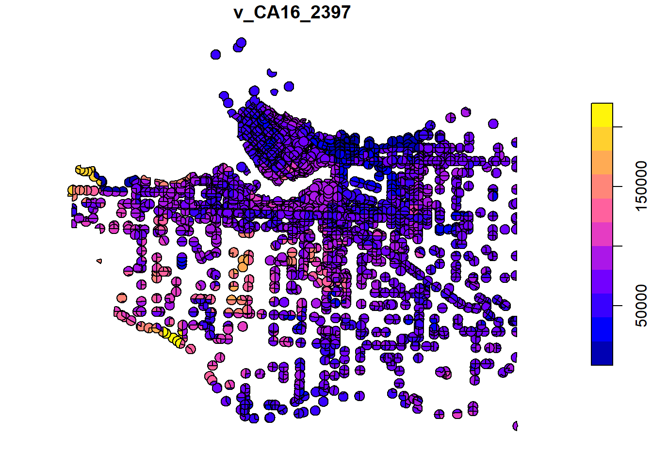
There are a lot of overlapping polygons in this dataset. Let’s simplify these data by averaging the census income data for each unique crash buffer. Recall that each icbc crash had a unique identifer we assigned it when we loaded it. The code below essentially is taking all of the different census data that overlapped with a crash buffer and averaging the income from that dissemination area. More formally, we can think about it as for each polygon that has the same uniqid, dissolve the geometry so that they all share the same extent and take the average value of v_CA16_2397 and assign it to the new geography. This will necessarily only leave 1 income value for each crash buffer, and “dissolve” the boundaries of buffers that were on the border of multiple census areas. This might make more sense by comparing the intersection plot with the dissolved/aggregated plot below.
average_income_by_crash_buffer <- intersect_van_census_crash_buffer %>%
  group_by(uniqid) %>%
  summarise(average_income = mean(v_CA16_2397,na.rm=TRUE))

plot(average_income_by_crash_buffer["average_income"])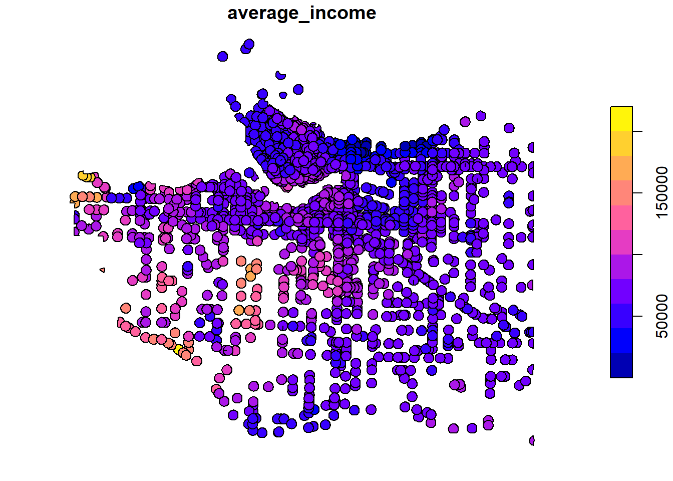
4.7 Spatial Joins
A spatial join will likely be one of the most common types of overlay analyses you will employ in your analyses. In a spatial join the goal is to combine the attribute data from one geographic dataset (the join dataset) and append it to the geometry of another geographic dataset (the target dataset), based on the spatial relationship between the two datasets (figure 4.7. In a spatial join, the join dataset typically has 1 to 2 more dimensions that of the target features (recall that polygons are 2 dimensional, lines are 1 dimensional and points are 0 dimensional).
Usually the goal in a spatial join is to summarize or aggregate attribute information of either points that fall on/within the geometry of polygon or line features, or, to summarize the attribute information of lines that fall within polygons. In a transportation safety context, a good example would be to aggregate crash point data to the neighbourhood it occured within (point-in-polygon), or the number of crashes that occur on a road segment (points-on-lines). Another transportation example would be to aggregate the road network features by neighbourhoods (lines-in polygons).
For example in Figure 4.7 we have the crash point map where each crash has an ID. We also have a neighbourhood map with the names of neighbourhoods. We want to join the neighbourhood names to the point data, based on the co-location of the points and the neighbourhoods. We define the crash points dataset as the “target dataset.” The target dataset is the one where we want to preserve the existing geometry and attributes. We define the neighbourhood polygon dataset as the “join dataset.” THe join dataset contains the attribute information we want to join to the attribute table of the target dataset. In short, when we run a spatial join we preserve the geometry of the target dataset and add the attribute information of the join dataset.
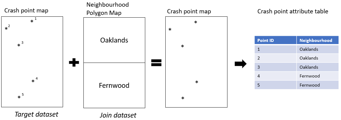
Figure 4.7: Diagram showing spatial join of polygons to points
ta.
In R we can use the st_join() function from the sf package to accomplish a spatial join. In this function the arguments that are input are st_join(x,y,join) where x refers to a target dataset (which needs to be an sf object), y refers to the join dataset. The default spatial relationship to use to define which feature attributes from the join dataset will be added to to which features from the target dataset is based on an intersection (i.e. st_intersects()). This can be modified to join attributes based on a different spatial relationship such as st_contains() or st_is_within_distance() among others. See the reference page for the full list.
Let’s go a through a few examples based on different purposes.
4.7.0.1 Points-in-polygon
In this example our end goal is to map the number of ICBC recorded bicycle crashes by dissemination area boundaries for the city of Vancouver. We will use the datasets we loaded earlier in the chapter:
vancouver_da_dep: Dissemination Area census geographies that include information on deprivation levels (see Attribute Join section above)icbc_crash_van: ICBC bicycle crash data for the City of Vancouver (see Buffer section above)
To enable counting of crashes within each dissemination area we are going to use a spatial join within a series of steps that will also draw upon what we learned about attribute joins and some data summary functionality from dplyr.
The first step is to join the DA level information to each point based on whether the point intersects with that polygon. Essentially, we want to take all of the DA level information and join it to each crash event based on the colocation of the crash and census data.
icbc_crash_van_join_da <- st_join(icbc_crash_van,vancouver_da_dep)
head(icbc_crash_van_join_da)
## Simple feature collection with 6 features and 49 fields
## Geometry type: POINT
## Dimension: XY
## Bounding box: xmin: 492170.9 ymin: 5458315 xmax: 494873.9 ymax: 5458438
## Projected CRS: NAD83 / UTM zone 10N
## # A tibble: 6 x 50
## `Crash Breakdown~ `Date Of Loss Ye~ `Crash Severity` `Cyclist Flag` `Day Of Week` `Derived Crash Cong~ `Intersection Cr~ `Month Of Year` `Motorcycle Fla~ `Municipality Nam~ `Parking Lot Fl~
## <chr> <dbl> <chr> <chr> <chr> <chr> <chr> <chr> <chr> <chr> <chr>
## 1 LOWER MAINLAND 2018 CASUALTY Yes SATURDAY SINGLE VEHICLE Yes MAY No VANCOUVER No
## 2 LOWER MAINLAND 2017 PROPERTY DAMAGE ~ Yes THURSDAY UNDETERMINED Yes MARCH No VANCOUVER No
## 3 LOWER MAINLAND 2015 CASUALTY Yes FRIDAY SINGLE VEHICLE Yes JUNE No VANCOUVER No
## 4 LOWER MAINLAND 2015 CASUALTY Yes WEDNESDAY SINGLE VEHICLE Yes JUNE No VANCOUVER No
## 5 LOWER MAINLAND 2016 CASUALTY Yes THURSDAY SINGLE VEHICLE Yes NOVEMBER No VANCOUVER No
## 6 LOWER MAINLAND 2019 PROPERTY DAMAGE ~ Yes WEDNESDAY SINGLE VEHICLE Yes JANUARY No VANCOUVER No
## # ... with 39 more variables: Pedestrian Flag <chr>, Region <chr>, Street Full Name (ifnull) <chr>, Time Category <chr>, Crash Breakdown <chr>, Cross Street Full Name <chr>,
## # Heavy Veh Flag <chr>, Mid Block Crash <chr>, Municipality Name <chr>, Municipality With Boundary <chr>, Road Location Description <chr>, Street Full Name <chr>, Crash Count <dbl>,
## # Number of Records <dbl>, geometry <POINT [m]>, uniqid <int>, Population <int>, Households <int>, GeoUID <chr>, Type <fct>, CD_UID <chr>, Shape Area <dbl>, Dwellings <int>, CSD_UID <chr>,
## # CT_UID <chr>, CMA_UID <chr>, Region Name <fct>, Area (sq km) <dbl>, v_CA16_2397 <dbl>, Province <chr>, Dissemination area (DA) Population <dbl>,
## # Ethno-cultural composition Quintiles <dbl>, Ethno-cultural composition Scores <dbl>, Situational vulnerability Quintiles <dbl>, Situational vulnerability Scores <dbl>,
## # Economic dependency Quintiles <dbl>, Economic dependency Scores <dbl>, Residential instability Quintiles <dbl>, Residential instability Scores <dbl>In the attribute table of our new object icbc_crash_van_join_da we can see that each point now has information for the dissemination area with which it is located (e.g. intersects with). A successful spatial join! But how do we go from here to map the number of crashes by dissemination area? The next step is to take our spatially joined data and use dplyr to group the data by the dissemination area unique identifier, add up the Crash Count variable for each row with the same unique id. Right now our data is still an sf point object. Now that the spatial join is done, we don’t need to keep the geometry associated with this feature so we can remove it using the st_drop_geometry() function. This will speed up the computation time for the functions performed on grouped data.
In the code chunk below we are grouping our data by the dissemination area unique id we just joined to our point data using the group_by() function and summing the Crash Count variable using the summarise() function.
no_icbc_crashes_by_da <-   icbc_crash_van_join_da %>%
  st_drop_geometry() %>%
  group_by(GeoUID) %>%
  summarise(total_crashes = sum(`Crash Count`))
The output is a table with one row for each dissemination area (unique GeoUID)
head(no_icbc_crashes_by_da)## # A tibble: 6 x 2
## GeoUID total_crashes
## <chr> <dbl>
## 1 59150310 1
## 2 59150311 1
## 3 59150313 4
## 4 59150329 3
## 5 59150330 1
## 6 59150332 1Now we have counts of crashes by the unique identifier of the dissemination area it occured in. Now we can simply join this table back to the polygon data using a left_join().
vancouver_da_dep_crashes <- left_join(vancouver_da_dep,no_icbc_crashes_by_da,by="GeoUID")


head(vancouver_da_dep_crashes)
## Simple feature collection with 6 features and 24 fields
## Geometry type: MULTIPOLYGON
## Dimension: XY
## Bounding box: xmin: 497754.1 ymin: 5458297 xmax: 498323.1 ymax: 5460083
## Projected CRS: NAD83 / UTM zone 10N
## Population Households GeoUID Type CD_UID Shape Area Dwellings CSD_UID CT_UID CMA_UID Region Name Area (sq km) v_CA16_2397 Province Dissemination area (DA) Population
## 1 632 254 59150307 DA 5915 0.29926 273 5915022 9330053.02 59933 Vancouver 0.29926 90965 British Columbia 669.4691
## 2 501 203 59150308 DA 5915 0.10956 223 5915022 9330053.02 59933 Vancouver 0.10956 93611 British Columbia 470.3942
## 3 745 269 59150309 DA 5915 0.11190 299 5915022 9330053.02 59933 Vancouver 0.11190 84736 British Columbia 728.7991
## 4 536 283 59150310 DA 5915 0.10940 310 5915022 9330053.02 59933 Vancouver 0.10940 45184 British Columbia 396.3275
## 5 532 181 59150311 DA 5915 0.08094 199 5915022 9330053.02 59933 Vancouver 0.08094 82517 British Columbia 623.7097
## 6 562 203 59150312 DA 5915 0.08706 211 5915022 9330053.02 59933 Vancouver 0.08706 74368 British Columbia 530.6063
## Ethno-cultural composition Quintiles Ethno-cultural composition Scores Situational vulnerability Quintiles Situational vulnerability Scores Economic dependency Quintiles
## 1 3 -0.2744621 2 -0.4505756 1
## 2 3 -0.2350062 1 -0.7415757 2
## 3 4 0.5496419 1 -0.6846734 2
## 4 4 0.8662144 5 0.3722661 2
## 5 4 0.6849209 2 -0.4435429 2
## 6 5 1.0570569 3 -0.2977577 1
## Economic dependency Scores Residential instability Quintiles Residential instability Scores total_crashes geometry
## 1 -0.9301352 4 0.1246316 NA MULTIPOLYGON (((498308 5459...
## 2 -0.6086799 2 -0.5748885 NA MULTIPOLYGON (((498301.6 54...
## 3 -0.6227231 3 -0.2030643 NA MULTIPOLYGON (((497939.5 54...
## 4 -0.4802208 5 1.9569124 1 MULTIPOLYGON (((498298.6 54...
## 5 -0.5483774 3 -0.4832458 1 MULTIPOLYGON (((498128.4 54...
## 6 -0.7775863 3 -0.1416693 NA MULTIPOLYGON (((498298.6 54...Our new column total_crashes has NA values for some polygons. This is because if a dissemination area did not have crashes occur within their boundaries they would not have been attribtued to a crash in our point dataset during the spatial join. The NA value actually then represents a 0. So let’s change the NA values to 0 using the replace_na() function from the tidyr package.
vancouver_da_dep_crashes <- vancouver_da_dep_crashes %>%
  mutate(total_crashes = replace_na(total_crashes,0))
Now let’s map the number of crashes from the new dataset vancouver_da_dep_crashes and overlay the original crash data icbc_crash_van
mapview(vancouver_da_dep_crashes,zcol = "total_crashes") + mapview(icbc_crash_van)4.7.0.2 Points-on-line
In a points-on-line spatial join we are applying the same concept as the previous example, but we instead want to join attribute data from line data to our point data. This type of operation is a bit trickier to implement because lines only 1-dimensions. So if a point does not fall exactly onto it’s geometry it is harder to join based on an intersection. There are a few ways around this as is the case with almost any kind of geoprocessing task. The simplest way would be to change spatial relationship from the default st_intersects to something like st_is_within_distance and specify a distance tolerance for considering a line to be attributed to a point. This is great if you are okay with a one-to-many spatial join where you create a new point object for every line segment within this distance. However, if we wanted to ensure a one-to-one join where you only join the attribute data from one line segment to one point - you will need to find a work around. One way to do this is to “snap” each point data to the nearest road segment, and then use the within st_join(x,y,join = st_is_within_distance, dist = tiny_value_like_1cm) to conduct the spatial join.
sf does not have a built in function for snapping points to nearest line segment but we can create one ourselves. Below is a function called st_snap_points() we define manually. It has 4 arguments, x for the point data, y for the line data, max_dist is the distance tolerance value, and namevar for specifying any uniqid from th original dataset. Feel free to ignore the details of the function below but make sure to run it before going through the rest of the section.
st_snap_points <- function(x, y, namevar, max_dist = 1000) {

  # this evaluates the length of the data
  if (inherits(x, "sf")) n = nrow(x)
  if (inherits(x, "sfc")) n = length(x)

  # this part:
  # 1. loops through every piece of data (every point)
  # 2. snaps a point to the nearest line geometries
  # 3. calculates the distance from point to line geometries
  # 4. retains only the shortest distances and generates a point at that intersection
  out = do.call("c",
                lapply(seq(n), function(i) {
                  nrst = st_nearest_points(st_geometry(x)[i], y)
                  nrst_len = st_length(nrst)
                  nrst_mn = which.min(nrst_len)
                  if (as.vector(nrst_len[nrst_mn]) > max_dist) return(st_geometry(x)[i])
                  return(st_cast(nrst[nrst_mn], "POINT")[2])
                })
  )

  # this part converts the data to a dataframe and adds a named column of your choice
  out_xy <- st_coordinates(out) %>% as.data.frame()
  out_xy <- out_xy %>%
    mutate({{namevar}} := x[[namevar]]) %>%
    st_as_sf(coords=c("X","Y"), crs=st_crs(x), remove=FALSE)

  return(out_xy)
}
Now that we have defined this function let’s try out another scenario. Similar to the section above, our end goal is to map the number of bicycle crashes (icbc_van_crash) that occur on the separated bicycle infrastructure network in Vancouver (bicycle_proj). The steps do so are as follows:
- Snap the crash locations to the nearest line segment based on a reasonable distance threshold using the
st_snap_pointsfunction - Perform a spatial join where we join the attributes of the nearest line segment to each point
- Aggregate the attribute data of the new spatially joined data by a unique identifier of the line segment
- Join the aggregated data back to the line segment data based on the unique identifier
Snap Points
Set a max distance of 20m to snap points. Outside of 20m then we don’t consider them occurring on an infrastructure segment and the position of the event will stay the same. This function may take a bit of time to run.
icbc_snp <- st_snap_points(x = icbc_crash_van,#crash van
                           y = bicycle_proj, #network infrasructure data
                           max_dist = 20,
                           namevar = "uniqid") #this only returns the geometry - doesn't preserve attributes

icbc_snp <-  left_join(icbc_snp,
                       icbc_crash_van %>%
                         st_drop_geometry(),
                       by = "uniqid")#return the attributes to the snapped locations


mapview(icbc_snp) + mapview(bicycle_proj)
Spatial Join
Now for each point let’s count the number of crashes that occur on that segment based on our 20m threshold. To do so we will join the unique id of the nearest road segment to the point data using st_join() and the st_within_distance() function. Since we already have snapped the points to the nearest road segment there is only one road segment assigned to each point and we specify a tiny distance to consider a spatial join.
icbc_snp_bicycle_inf <- st_join(icbc_snp,
                         bicycle_proj["osm_id"], #select only the column "osm_id"
                           join = st_is_within_distance, dist = 0.001) #for each point assign the LIXID that it falls on by indicating a very small distance tolerance (here it is 1mm)


icbc_snp_bicycle_inf %>%
  select(uniqid,`Crash Count`,osm_id) # look at the results
## Simple feature collection with 3405 features and 3 fields
## Geometry type: POINT
## Dimension: XY
## Bounding box: xmin: 484327.3 ymin: 5449979 xmax: 498329.2 ymax: 5462021
## Projected CRS: NAD83 / UTM zone 10N
## First 10 features:
## uniqid Crash Count osm_id geometry
## 1 42 1 <NA> POINT (492170.9 5458438)
## 2 43 1 368058222 POINT (492279.2 5458372)
## 3 45 1 <NA> POINT (492940 5458424)
## 4 46 1 368210443 POINT (494873.4 5458316)
## 5 47 1 368210443 POINT (494873.4 5458316)
## 6 48 1 368058222 POINT (492279.2 5458372)
## 7 51 1 748846437 POINT (490680.9 5458413)
## 8 52 1 <NA> POINT (492170.9 5458438)
## 9 56 1 827958314 POINT (491713.7 5458318)
## 10 57 1 540329767 POINT (490452.9 5458326)Note how only the points that were snapped to bicycle infrastructure locations have a uniqid assigned from the bicycle infrastructure data. The NA values indicate no lines were within a distance of 0.001 meters (i.e. equivalent to 20m since we snapped the points to the nearest segment based on a 20m threshold)
Spatial Aggregation
Now let’s count the number of points with same osm_id.
no_crashes_by_osm_id <- icbc_snp_bicycle_inf %>%
  group_by(osm_id) %>%
  summarise(n_crashes = sum(`Crash Count`)) %>%
  st_drop_geometry() # drop the geometry from this - we only need the uniqid for the bicycle infrastrucutre data and the counts
Attribute Join
Now we can join this data back to the bicycle infrastructure polyline data. Polylines without any crashes will be assigned an NA value because they don’t have a matching record in the join. We then simply replace the NA values with a 0 after the join using the replace_na() from the tidyr package.
bicycle_infra_crash_count <- left_join(bicycle_proj,no_crashes_by_osm_id , by = "osm_id") %>%
  mutate(n_crashes = replace_na(n_crashes,0))
Let’s map out the number of crashes by bicycle infrastructure and layer on the original point data and zoom into areas with collision events and see if the results make sense.
mapview(bicycle_infra_crash_count,zcol="n_crashes") + mapview(icbc_snp)4.7.0.3 Lines-in-polygon
Here let’s assume a scenario where the end goal is to calculate the length of separated bicycle infrastructure within each dissemination area in the City of Vancouver. Recall we created the following datasets from earlier in the chapter:
bicycle_proj: separated bicycle infrastructure polylines for the City of Vancouver in UTM Zone 10Nvancouver_da_dep: dissemination area boundaries for the City of Vancouver in UTM Zone 10N
The main problem is that as of now, the line segments for bicycle infrastructure do not line up with the boundary of disseminatin areas. This concept is illustrated in the left panel of Figure 4.7 where we have one polyline that crosses multiple boundaries. We need to cut the line segments where they intersect with the boundaries of dissemination areas such as in Figure 4.7 using st_intersection() so that we can then calculate the length of each individual segment using st_length().
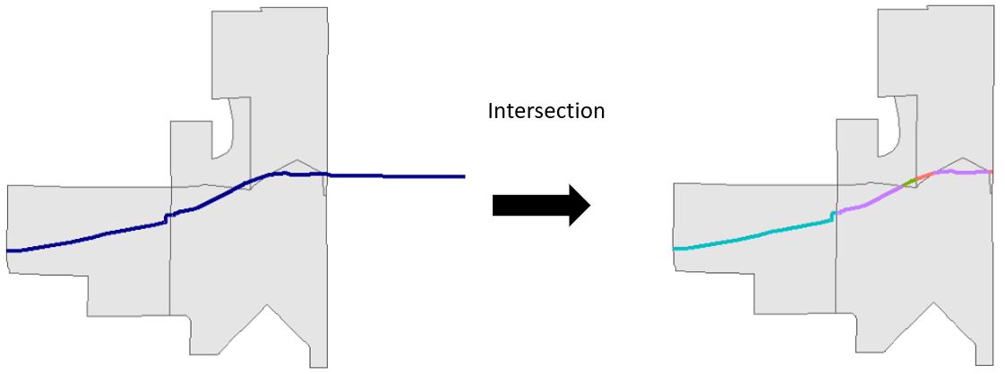
Figure 4.8: Intersection of a single polyline (blue) by polygons (grey)
From there we can sum the length of each line segment by the dissemination area’s unique identfier (GeoUID) in a few different ways, including a spatial join. Let’s try this out so we can see some of the problems that can arise with this type of data and operation.
First, let’s create the “cut” version of our bicycle infrastructure layer using st_intersection(). I am going to do this with subsets of original datasets that only contain the unique identifier as attribute data to make our data exploration a little cleaner.
## Warning: attribute variables are assumed to be spatially constant throughout all geometriesWe can then calculate the length of each line segment using a function called st_length().
bicycle_cut <- bicycle_cut %>%
  mutate(length_m = st_length(.))

bicycle_cut
## Simple feature collection with 1473 features and 3 fields
## Geometry type: GEOMETRY
## Dimension: XY
## Bounding box: xmin: 483720 ymin: 5449700 xmax: 498317.2 ymax: 5462376
## Projected CRS: NAD83 / UTM zone 10N
## First 10 features:
## osm_id GeoUID geometry length_m
## 35260598 35260598 59150307 LINESTRING (498105.5 545987... 157.80005 [m]
## 35260599 35260599 59150307 LINESTRING (497911 5459475,... 32.86117 [m]
## 36691655 36691655 59150307 LINESTRING (497911 5459475,... 163.86383 [m]
## 41840546 41840546 59150307 LINESTRING (498180.4 545988... 76.01887 [m]
## 75573893 75573893 59150307 LINESTRING (498226.7 545987... 44.49847 [m]
## 210638528 210638528 59150307 LINESTRING (498190.6 545997... 84.65905 [m]
## 210638530 210638530 59150307 LINESTRING (498235.3 545998... 46.27267 [m]
## 336365962 336365962 59150307 LINESTRING (497942.1 545946... 56.43094 [m]
## 340103260 340103260 59150307 LINESTRING (497944.5 545952... 86.09529 [m]
## 380516622 380516622 59150307 LINESTRING (498317.2 545999... 84.11612 [m]Notice how the intersection also attributed the GeoUID from the Dissemination Area boundary. We could then use that information to summarise the length of polylines within each GeoUID.
But let’s take a look at our data.
mapview(bicycle_cut) + mapview(vancouver_da_sub)Note how some bicycle infrastructure line segments follow the border of dissemination areas. One of the problems with trying to summarise transportation data within census polygons is that often the boundaries of census areas follow roads! So technically a given road belongs to more than one dissemination area. The intersection we performed above only assigned the attribute data from the neighbourhoods that intersected with a given road, a one-to-one spatial join. One way to deal with this would be to use the st_within_distance within st_join and create a polyline for each dissemination area that is within a certain distance of a line segment. This is called a one-to-many spatial join that will create multiple line segments for each dissemination where that spatial relationship is true. Let’s try it. If a line segment is within 5 metres of a dissemination area, join the attribute data from that dissemination area to the line segment. I chose 5 m to allow for some inaccuracy in the way the line data were digitized (e.g. a line segment may suppose to follow a boundary exactly but is actually a few metres off to one side etc.)
cut_join_da <- st_join(bicycle_cut, vancouver_da_sub,join = st_is_within_distance,dist=5)

cut_join_da
## Simple feature collection with 2585 features and 4 fields
## Geometry type: GEOMETRY
## Dimension: XY
## Bounding box: xmin: 483720 ymin: 5449700 xmax: 498317.2 ymax: 5462376
## Projected CRS: NAD83 / UTM zone 10N
## First 10 features:
## osm_id GeoUID.x length_m GeoUID.y geometry
## 35260598 35260598 59150307 157.80005 [m] 59150307 LINESTRING (498105.5 545987...
## 35260598.1 35260598 59150307 157.80005 [m] 59153215 LINESTRING (498105.5 545987...
## 35260599 35260599 59150307 32.86117 [m] 59150307 LINESTRING (497911 5459475,...
## 36691655 36691655 59150307 163.86383 [m] 59150307 LINESTRING (497911 5459475,...
## 41840546 41840546 59150307 76.01887 [m] 59150307 LINESTRING (498180.4 545988...
## 75573893 75573893 59150307 44.49847 [m] 59150307 LINESTRING (498226.7 545987...
## 210638528 210638528 59150307 84.65905 [m] 59150307 LINESTRING (498190.6 545997...
## 210638530 210638530 59150307 46.27267 [m] 59150307 LINESTRING (498235.3 545998...
## 336365962 336365962 59150307 56.43094 [m] 59150307 LINESTRING (497942.1 545946...
## 340103260 340103260 59150307 86.09529 [m] 59150307 LINESTRING (497944.5 545952...Note how the first two rows of our data have the same osm_id but different values for GeoUID.y. What this means is that for this particular line segment there are multiple dissemination areas that fullfill the spatial join criteria (is within 5 metres). Now we let’s summarise the length_m column by the GeoUID.y column.
length_by_da <- cut_join_da %>%
  st_drop_geometry() %>%
  group_by(GeoUID.y) %>%
  summarise(total_length_km = sum(as.numeric(length_m))/1000)

head(length_by_da)
## # A tibble: 6 x 2
## GeoUID.y total_length_km
## <chr> <dbl>
## 1 59150307 1.34
## 2 59150309 0.218
## 3 59150312 0.0560
## 4 59150313 0.0939
## 5 59150328 0.171
## 6 59150329 1.30Now let’s join this back to our dissemination area boundaries, replace the NAs with 0s and map the results!
vancouver_da_sub <- left_join(vancouver_da_sub,length_by_da , by = c("GeoUID"="GeoUID.y")) %>%
  mutate(total_length_km = replace_na(total_length_km,0))

vancouver_da_sub
## Simple feature collection with 993 features and 2 fields
## Geometry type: MULTIPOLYGON
## Dimension: XY
## Bounding box: xmin: 483690.9 ymin: 5449535 xmax: 498329.2 ymax: 5462381
## Projected CRS: NAD83 / UTM zone 10N
## First 10 features:
## GeoUID total_length_km geometry
## 1 59150307 1.33568195 MULTIPOLYGON (((498308 5459...
## 2 59150308 0.00000000 MULTIPOLYGON (((498301.6 54...
## 3 59150309 0.21754280 MULTIPOLYGON (((497939.5 54...
## 4 59150310 0.00000000 MULTIPOLYGON (((498298.6 54...
## 5 59150311 0.00000000 MULTIPOLYGON (((498128.4 54...
## 6 59150312 0.05595795 MULTIPOLYGON (((498298.6 54...
## 7 59150313 0.09386538 MULTIPOLYGON (((498259 5458...
## 8 59150328 0.17094843 MULTIPOLYGON (((498102 5458...
## 9 59150329 1.29789720 MULTIPOLYGON (((497801.1 54...
## 10 59150330 0.00000000 MULTIPOLYGON (((497312 5458...mapview(vancouver_da_sub,zcol = "total_length_km") + mapview(bicycle_sub)We could also map the density instead:
vancouver_da_sub <- vancouver_da_sub %>%
  mutate(total_area_km2 = as.numeric(st_area(.)/1000/1000),
         total_bike_dens = total_length_km/ total_area_km2
         )

mapview(vancouver_da_sub,zcol = "total_bike_dens")  + mapview(bicycle_sub)