Chapter 3 Geographic Vector and Raster Data with R
In the previous chapter you were introduced to the concepts of vector and raster data, and developed some intuition on their structure and how they might be typically used in a GIS setting. Now we are going to get into the nuts and bolts of how these data types are structured in R using the sf package (Pebesma 2021) to create our own vector data, and the raster package to create our own raster data (Hijmans 2020). This exercise is designed to get you familiar with the different types of geographic data and how they work in R. In reality as applied researchers you will be much more likely to be downloading various different spatial data from different sources and combining them in different ways to answer specific research questions. After we go through making up our own spatial data, we will load and map existing spatial datasets.
This chapter requires the following packages:
library(sf)
library(raster)
library(crsuggest)
library(osmdata)
library(cancensus)
library(readr)
library(dplyr)
3.1 Vector Data
The sf package can be used to represent different geometry types in R. In this tutorial we will focus on three simple types of geometry: points, linestrings (i.e. lines) and polygons. There are 14 additional types of geometry that can be represented in sf which for now we can ignore but are detailed in the sf vignette.
As mentioned in the previous chapter, vector data are used to represent an object (or feature) that occurs somewhere on Earth that has some kind of spatial geometry. Here spatial geometry refers the idea that each feature has a shape that can be described by at least one two-dimensional (x,y) coordinate that references a specific location on earth. The simplest geometry for a spatial object is a point, where each feature has a single XY coordinate (Figure 3.1A). A line feature consists of two connected vertices whose location is defined by a single XY coordinate (Figure 3.1B). A polygon feature consists of at least three XY coordinates that are fully enclosed (Figure 3.1C).
- Points are 0-dimensional in that they have no measurable length or area.
- Lines are 1-dimensional in that they one can measure its length, but cannot measure its area.
- A polygon is 2-dimensional as you can measure both its length and its area.
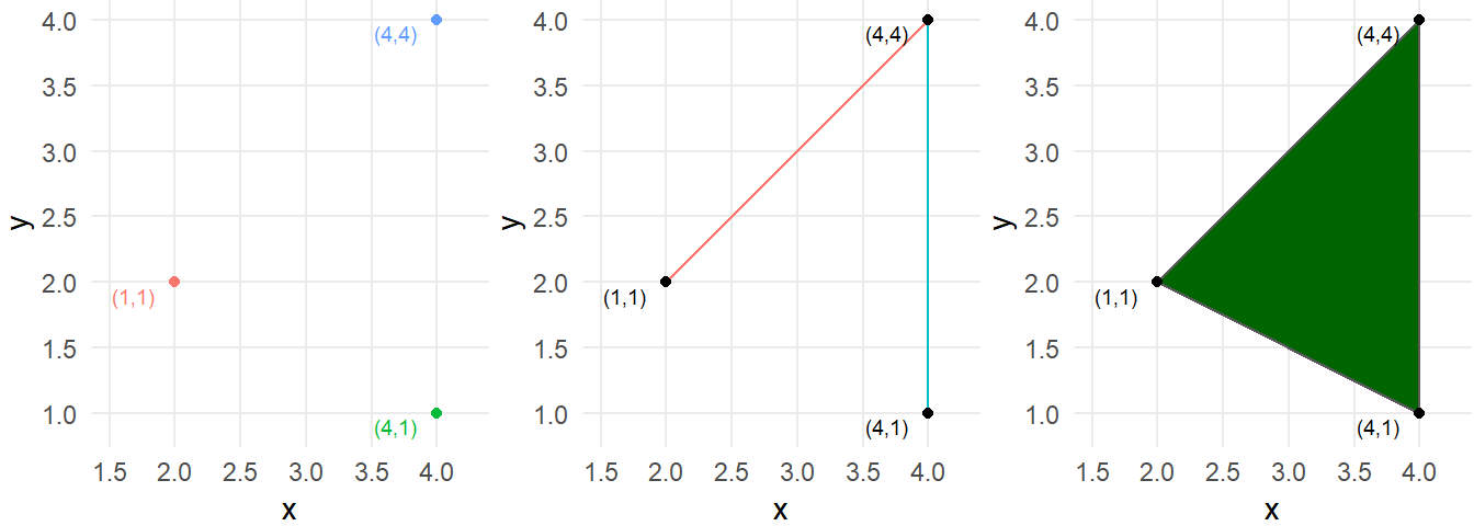
Figure 3.1: A) Three point features each with their own XY coordinate. B) Two line features defined by connecting two XY coordinates. C) One polygon feature defined by three XY coordinates.
Now we are going to go through each of the three geometry types as they are represented in the sf package and create our own data. The thing I want to impress upon you at this stage it is more important to follow along and try to understand the concepts than it is to memorize any of these terms. You will inevitably need to go back and look things up as you progress your GIS skills but here I just want to introduce how these data are structured in a step-by-step way without getting to complicated to quickly (hopefully). I’ve always learned best through doing so I’d encourage you to follow along in your own R script and play around with code as you go through. Let’s get started.
3.1.1 Points
First we are going to create our own point data. In sf we can input XY coordinates into the st_point() function to create point data. Here is a good place to clarify some confusing terminology. In R programming a “vector” is a basic data structure which contains a sequence of values of the same data type (e.g. numeric, character, factor) and can be created using the c() function. This can be distinguished from geographic vector data we have been just discussing. When referring the R data structure known as a vector I will call it an R vector. So let’s get started! Open up an R script and run the lines of code below.
a_single_point <- st_point(x = c(1,3)) # a single point with XY coordinates of 1,3 in unspecified coordinate system
a_single_point # view the content of the object
## POINT (1 3)attributes(a_single_point) #view the different components of an sfg object## $class
## [1] "XY" "POINT" "sfg"In the code chunk above I create a spatial object called a_single_point using a function st_point() from the sf package. The function takes a single R vector as its argument with two numeric data elements corresponding to the X and Y coordinate. The R vector c(1,3) specifies a point whose x coordinate is 1 and and the y coordinate is 3.
The st_point() function outputs a simple feature geometry (sfg) object with geometry type POINT. An sfg object is a spatial object that only stores XY coordinate information and does not have any information on the geographic coordinate system, datum or projection those coordinates are in, nor does it have any other attribute data associated with that point. Furthermore st_point() can only store a single point object.
What if we wanted to create an sfg object with more than one point? To do so we will need to use another function to build on the sfg object and create what’s called a simple feature geometry column object (sfc) using the st_sfc() function. An sfc object can store any number of sfg objects, as well as information on the coordinate reference system.
#create five sfg point objects
point1 <- st_point(x = c(1,3))
point2 <- st_point(x = c(2, 4))
point3 <- st_point(x = c(3, 3))
point4 <- st_point(x = c(4, 3))
point5 <- st_point(x = c(5, 2))

points <- st_sfc(point1,point2,point3,point4,point5) # create a single sfc points object

points
## Geometry set for 5 features
## Geometry type: POINT
## Dimension: XY
## Bounding box: xmin: 1 ymin: 2 xmax: 5 ymax: 4
## CRS: NA## POINT (1 3)## POINT (2 4)## POINT (3 3)## POINT (4 3)## POINT (5 2)In the code chunk above I created multiple sfg points, inputted each into the st_sfc() function to create a single sfc object to store all the point data. Note how it now the object now has space to store information on the overall spatial extent as represented by the bbox attribute (bbox stands for bounding box which has information on the smallest rectangle that would encompass all elements in the data), as well as space for information on something called a “CRS.” CRS stands for Coordinate Reference System (e.g.the information on the geographic coordinate system and map projection associated with our x and y coordinates). Right now our points data have an undefined coordinate system. For the sake of the example, let’s say that we built these data based on longitude and latitude coordinates using a very commonly used geographic coordinate system called WGS84. We could then input this information into the points object using the corresponding EPSG code of 4326. An EPSG code are 4-5 digit numbers that represent a single CRS.
points_wgs <- st_sfc(point1,point2,point3,point4,point5,crs=4326) # create a single sfc points object, and define the CRS

points_wgs
## Geometry set for 5 features
## Geometry type: POINT
## Dimension: XY
## Bounding box: xmin: 1 ymin: 2 xmax: 5 ymax: 4
## Geodetic CRS: WGS 84## POINT (1 3)## POINT (2 4)## POINT (3 3)## POINT (4 3)## POINT (5 2)Now we can see that the points object has a defined CRS! If we examine the components of the points_wgs object we can see all the details of the WGS1984 CRS in the CRS component of the object.
attributes(points)## $class
## [1] "sfc_POINT" "sfc"
##
## $precision
## [1] 0
##
## $bbox
## xmin ymin xmax ymax
## 1 2 5 4
##
## $crs
## Coordinate Reference System: NA
##
## $n_empty
## [1] 0Let’s quickly plot the point data using the plot() function. This function does not allow for a lot of flexibility in creating maps. We will get into more detail on how to map out spatial data in R later in the tutorial.
plot(points_wgs,col="red",pch=16) # map the sfc object using the plot function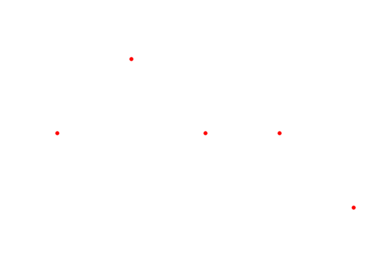
The one notable missing component from sfc is that there is no space for attribute data. Attribute data refers to any number of characteristics or attributes associated with any given feature in a vector dataset. For example, let’s say that the points we just created actually represented the location of traffic crash injuries and for each injury we had information on the mode of transport of the victim. Because the sfg objects can’t store attribute information, we need to create a simple feature (sf) object which can integrate both the location and the attribute data.
To create an sf object we use the function st_sf(). First though let’s create the attribute data. Below we create a data.frame with one column and five rows. The order of the rows corresponds to the order of the rows in the points_wgs object.
points_attribute_data <- data.frame(transport_mode = c("Bicycle","Pedestrian","Motor Vehicle","Motor Vehicle","Motor Vehicle"))

points_attribute_data
## transport_mode
## 1 Bicycle
## 2 Pedestrian
## 3 Motor Vehicle
## 4 Motor Vehicle
## 5 Motor VehicleIn the points_attribute_data data frame we specify that for the first point the injured victim was a bicyclist, the second the victim was a pedestrian, and the remaining three were motor vehicle users.
We can then associate the attribute data with the spatial points data using the st_sf() function and use the plot() function which will automatically map out the attribute features of an sf object. Again, this is fine for now but we will introduce better ways to create maps in R as we progress through the tutorial.
points_sf <- st_sf(points_attribute_data,geometry=points)

points_sf
## Simple feature collection with 5 features and 1 field
## Geometry type: POINT
## Dimension: XY
## Bounding box: xmin: 1 ymin: 2 xmax: 5 ymax: 4
## CRS: NA
## transport_mode geometry
## 1 Bicycle POINT (1 3)
## 2 Pedestrian POINT (2 4)
## 3 Motor Vehicle POINT (3 3)
## 4 Motor Vehicle POINT (4 3)
## 5 Motor Vehicle POINT (5 2)plot(points_sf,pch=16)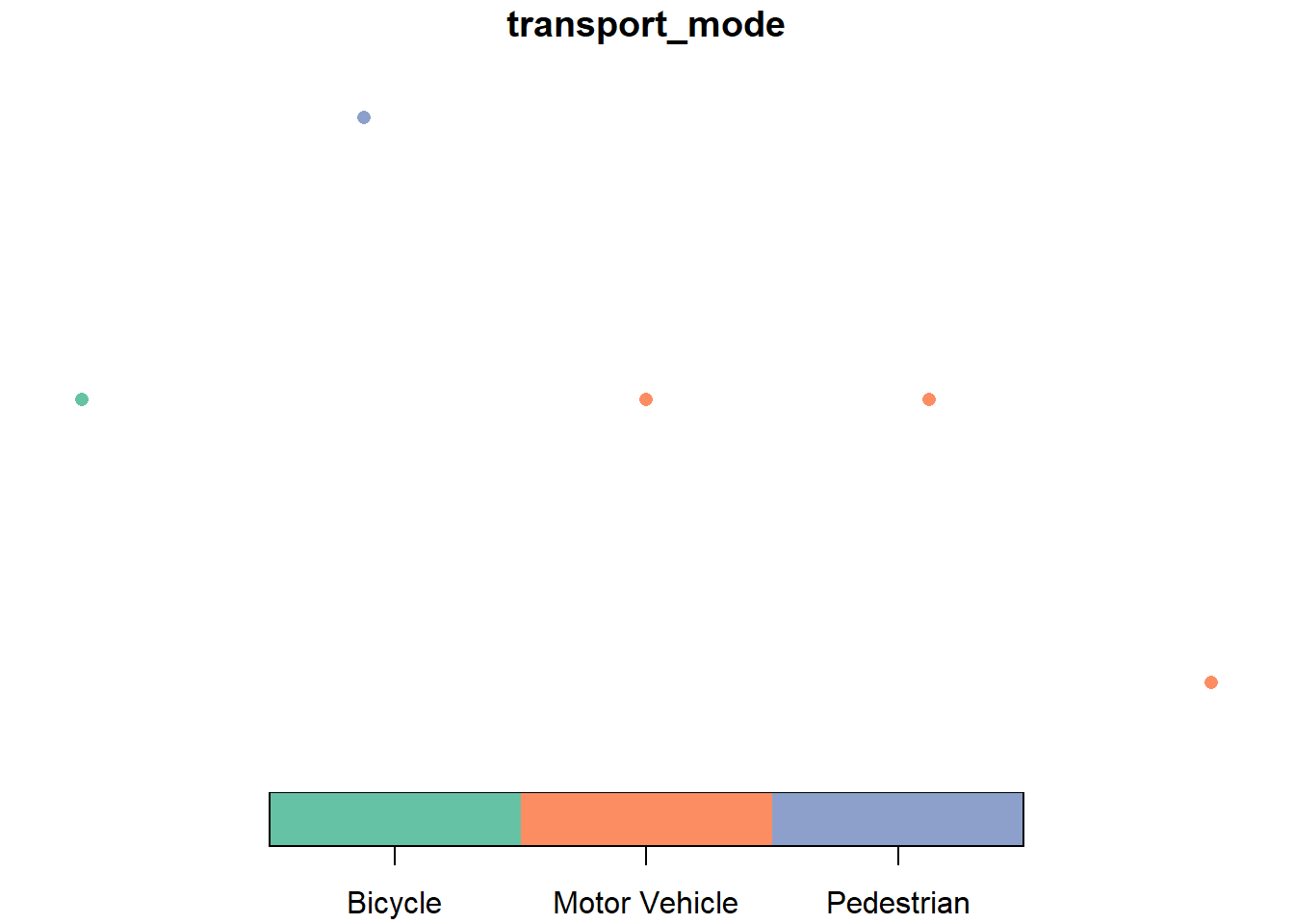
3.1.2 Lines
Here we can repeat the same process as above: creating an sfg, sfc and sf object but for the LINESTRING geometry. The st_line() function takes a matrix with at least two XY coordinates. A matrix is a essentially a two-dimensional version of an R vector. We can create a matrix that represents a single line by defining the nodes of the line in a series of R vectors and appending them by row using the function rbind().
a_single_line_matrix <- rbind(c(1,1),
                             c(2, 4),
                             c(3, 3),
                             c(4, 3),
                             c(5,2))# create a matrix with

a_single_line_matrix
## [,1] [,2]
## [1,] 1 1
## [2,] 2 4
## [3,] 3 3
## [4,] 4 3
## [5,] 5 2The matrix represents the XY coordinates of each vertex in the line segment, with the first column representing the X coordinates, and the second representing the Y coordinates
a_single_line <- st_linestring(a_single_line_matrix)
a_single_line## LINESTRING (1 1, 2 4, 3 3, 4 3, 5 2)attributes(a_single_line)## $dim
## [1] 5 2
##
## $class
## [1] "XY" "LINESTRING" "sfg"plot(a_single_line,col="darkblue")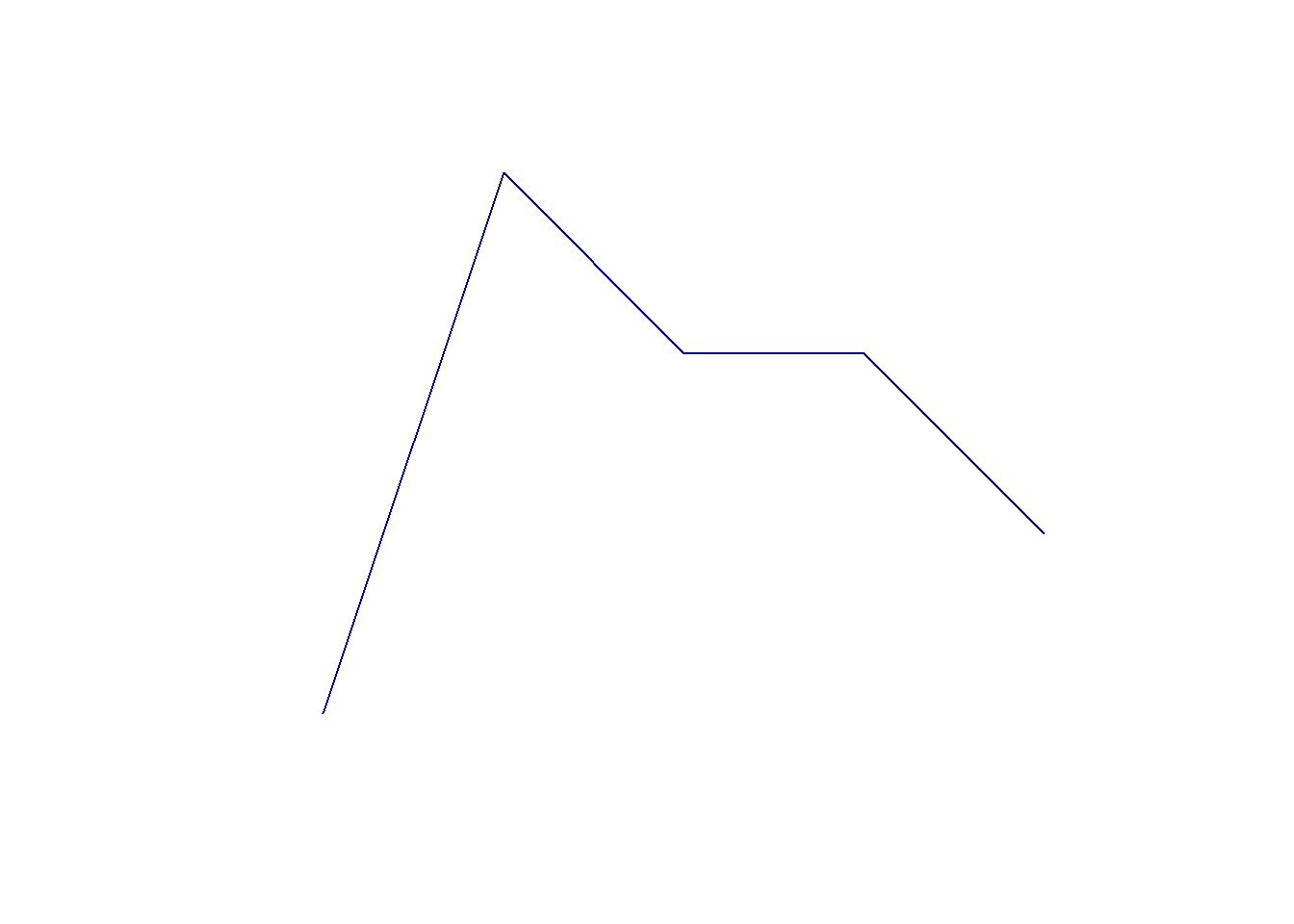
Now let’s create an sfc object with information on the associated CRS by creating and inputting multiple sfg linestring objects and the CRS code of 4326 corresponding to WGS 1984.
line1 <- st_linestring(rbind(c(1,1),
c(2,4),
c(3,3),
c(4,3),
c(5,2)))
line2 <- st_linestring(rbind(c(3,3),
c(3,5),
c(4,5)))
line3 <- st_linestring(rbind(c(2,4),
c(-1,4),
c(-2,-2)))
lines <- st_sfc(line1,line2,line3,crs=4326)
lines## Geometry set for 3 features
## Geometry type: LINESTRING
## Dimension: XY
## Bounding box: xmin: -2 ymin: -2 xmax: 5 ymax: 5
## Geodetic CRS: WGS 84## LINESTRING (1 1, 2 4, 3 3, 4 3, 5 2)## LINESTRING (3 3, 3 5, 4 5)## LINESTRING (2 4, -1 4, -2 -2)plot(lines)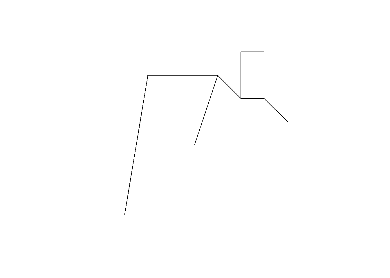
Let’s say each line represents a different road segment, each of which has a different name and speed limit. Let’s create the attribute table to reflect this:
line_attribute_data <- data.frame(road_name = c("Vinmore Avenue","Williams Road","Empress Avenue"),
speed_limit = c(30,50,40))
line_attribute_data## road_name speed_limit
## 1 Vinmore Avenue 30
## 2 Williams Road 50
## 3 Empress Avenue 40Then let’s attach the geometry to the attribute table.
lines_sf <- st_sf(line_attribute_data,geometry=lines)
lines_sf## Simple feature collection with 3 features and 2 fields
## Geometry type: LINESTRING
## Dimension: XY
## Bounding box: xmin: -2 ymin: -2 xmax: 5 ymax: 5
## Geodetic CRS: WGS 84
## road_name speed_limit geometry
## 1 Vinmore Avenue 30 LINESTRING (1 1, 2 4, 3 3, ...
## 2 Williams Road 50 LINESTRING (3 3, 3 5, 4 5)
## 3 Empress Avenue 40 LINESTRING (2 4, -1 4, -2 -2)Let’s then map out these data using the plot() function again.
plot(lines_sf)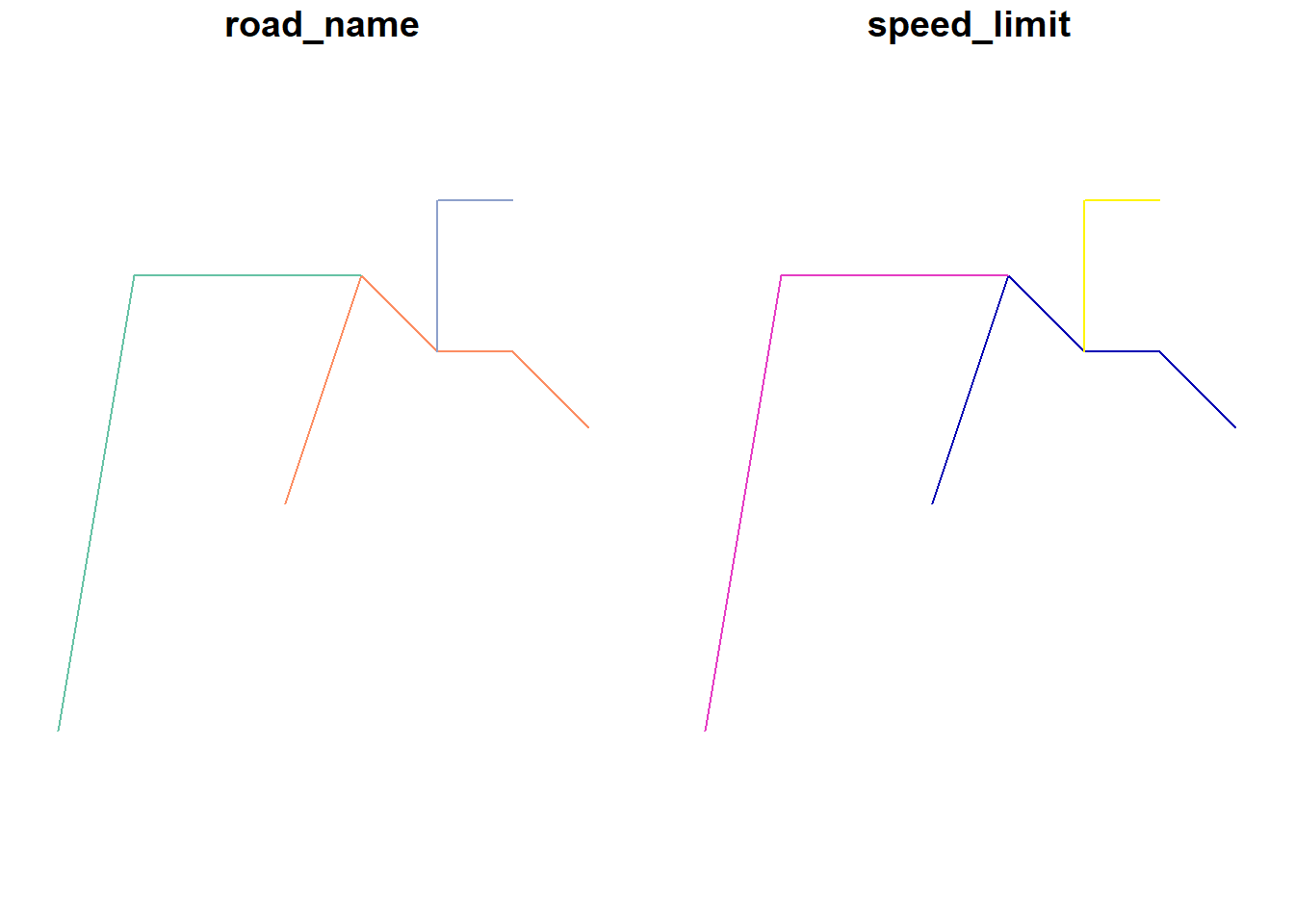
The plot() function will automatically map out the attributes of each segment given an sf object is input to it. We can clearly see the three different LINESTRING geometries representing different roads. If we want to map a specific attribute we need to specify it using the [] notation:
plot(lines_sf[1])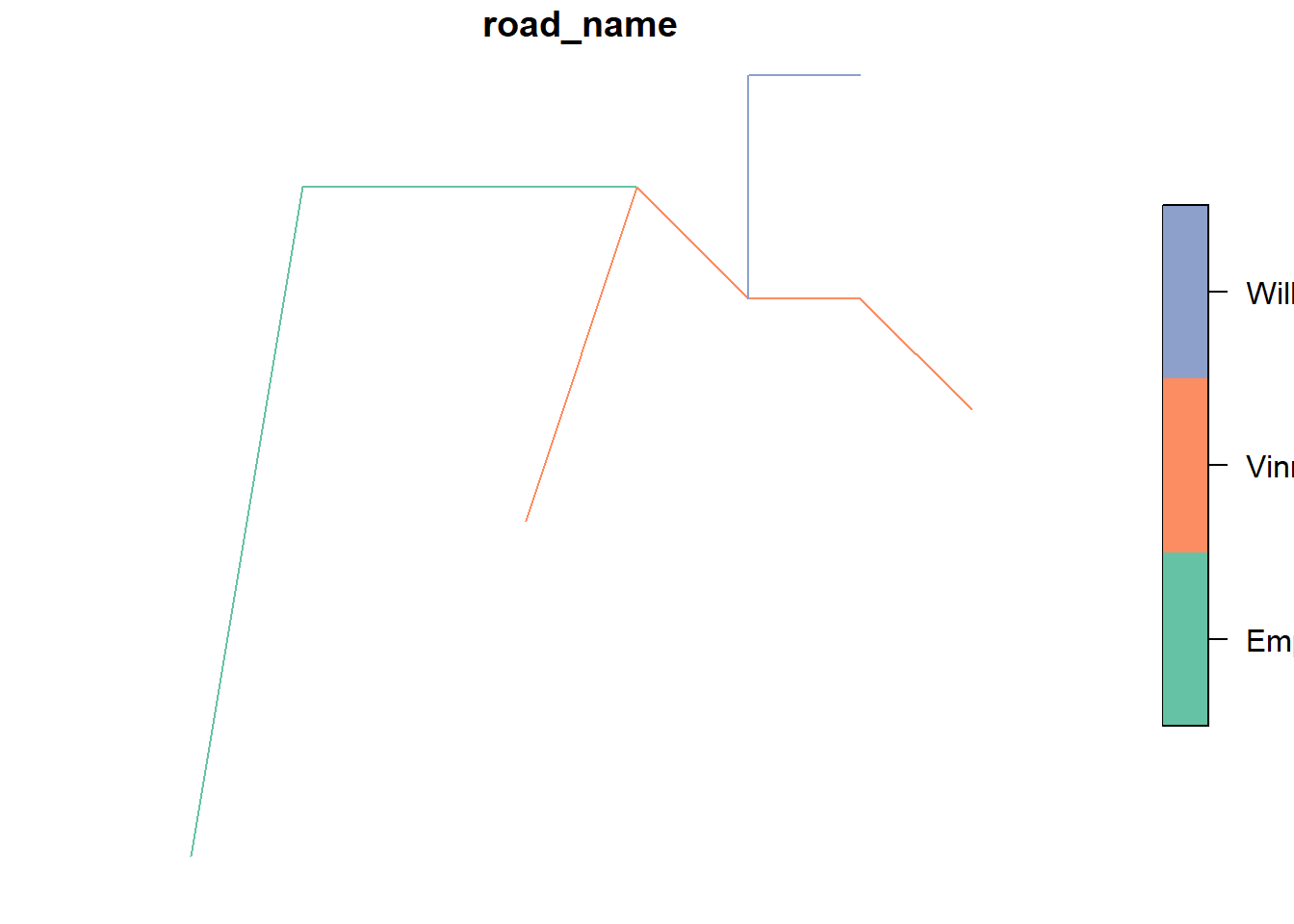
plot(lines_sf["speed_limit"])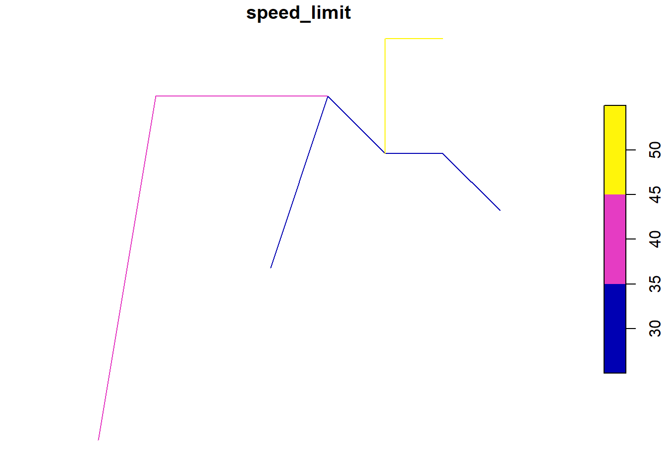
3.1.3 Polygons
Recall that a polygon is essentially an enclosed linestring (e.g. a linestring whose first and last vertex is the same coordinate). In sf an sfg object with POLYGON geometry is created through the st_polygon() function. The function takes a list as an argument which contains a linestring matrix where the first and last rows are the same XY coordinate within a list element.
a_polygon_vertices_matrix <- rbind(c(1,1), c(2, 4), c(3, 3), c(4, 3), c(5,2),c(1,1))
a_polygon_list = list(a_polygon_vertices_matrix)
a_polygon_list## [[1]]
##      [,1] [,2]
## [1,]    1    1
## [2,]    2    4
## [3,]    3    3
## [4,]    4    3
## [5,]    5    2
## [6,] 1 1a_polygon <- st_polygon(a_polygon_list)
plot(a_polygon,col="forestgreen")
We can create a more complex polygon with a hole by creating another polygon whose vertices occur within the first polygon, and adding it to the list(). Let’s say this POLYGON object represents the extent of a forest, and we wish to remove the boundaries of the lake that occurs within it.
lake_vertices_matrix <- rbind(c(1.5, 1.5),c(1.5,1.75),c(1.75,1.75),c(1.75,1.5),c(1.5,1.5))
lake_vertices_matrix
## [,1] [,2]
## [1,] 1.50 1.50
## [2,] 1.50 1.75
## [3,] 1.75 1.75
## [4,] 1.75 1.50
## [5,] 1.50 1.50a_single_polygon_with_a_hole_list = list(a_polygon_vertices_matrix,lake_vertices_matrix)
a_single_polygon_with_a_hole_list## [[1]]
## [,1] [,2]
## [1,] 1 1
## [2,] 2 4
## [3,] 3 3
## [4,] 4 3
## [5,] 5 2
## [6,] 1 1
##
## [[2]]
##      [,1] [,2]
## [1,] 1.50 1.50
## [2,] 1.50 1.75
## [3,] 1.75 1.75
## [4,] 1.75 1.50
## [5,] 1.50 1.50a_single_polygon_with_a_hole <- st_polygon(a_single_polygon_with_a_hole_list)
plot(a_single_polygon_with_a_hole,col="forestgreen")
Now let’s create an sf object with multiple polygons, attribute information and a defined CRS. Let’s say we have two polygons each representing a the boundaries of different parks in a city.
park1 <- a_single_polygon_with_a_hole
park2 <- st_polygon(list(
  rbind(
    c(6,6),c(8,7),c(11,9), c(10,6),c(8,5),c(6,6)
  )
))

park_attributes <- data.frame(park_name = c("Gilmore","Dixon"))

parks_sf <- st_sf(park_attributes, geometry = st_sfc(park1,park2,crs=4326))

plot(parks_sf)
Okay! So that is the basics of representing geographic vector data in R using the sf package. To summarize there are three types of data structures:
sfgobjects store XY information on a single feature geometry includingPOINT,LINESTRING, ANDPOLYGONsfcobjects store manysfgobjects as well as information on the coordinate system the XY information refers tosfobjects can store attribute data in addition to the spatial information represented in thesfc
Ultimately, in your research you will only really need to worry about sf objects. You will be hard pressed to find a situation where you need to create your own vector data from scratch in this manner. This was an exercise aimed at learning how the different geographic data types are structured in sf so that you’ll have a good understanding of the data you import from other sources, or when you convert tabular latitude and longitude event data into spatial point data (often spatial point data are initially available only in spreadsheet format!).
3.2 Raster
Let’s now take a bit of a deeper dive into raster data. Raster data are, fortunately, a lot simpler than vector data. Raster data are composed of a grid with equally spaced cells which cover some extent on the earths surface. Each cell can store one numeric value which can correspond to any measurable quantity you can think of including both categorical and numerical concepts. For example, raster data can be used to represent land cover types (categories such as forest, built up areas, or wetlands etc. ) or average annual precipitation.
The key parameter for raster data is its spatial resolution, that is, how small or large the cells of the grid are. Higher spatial resolution indicates a smaller cell size. Let’s explore raster data using the raster package and create some of our own data.
First let’s assume our study area is the City of Vancouver and we have our data in the CRS known as NAD 83 UTM Zone 10N (EPSG = 26910). In a UTM projection coordinates are specified in metres from a central meridian (eastings) and from the equator(northings). The extent of the study area in eastings and northings is from east to west 483,691 to 498,329 metres and from north to south 5,449,535 to 5,462,381. We want our spatial resolution to be 10000 m\(^2\) (100 x 100 grid cells)
van_raster <- raster(resolution=1000, #specify spatial resolution
                     xmn=483691, xmx=498329, #specify extent from east to west in metres
                     ymn=5449535, ymx=5462381, #specify extent from north to south in metres
                     crs=26910) #set projection
van_raster
## class : RasterLayer
## dimensions : 13, 15, 195 (nrow, ncol, ncell)
## resolution : 1000, 1000 (x, y)
## extent : 483691, 498691, 5449381, 5462381 (xmin, xmax, ymin, ymax)
## crs : +proj=utm +zone=10 +datum=NAD83 +units=m +no_defsUsing the raster() function and specifiying some key parameters we have created a RasterLayer object that is a rectangular grid cell with each cell being 10m by 10m in size, that covers the extent of the City of Vancouver. But we are missing a key component, the values of the grid cells!
values(van_raster)## [1] NA NA NA NA NA NA NA NA NA NA NA NA NA NA NA NA NA NA NA NA NA NA NA NA NA NA NA NA NA NA NA NA NA NA NA NA NA NA NA NA NA NA NA NA NA NA NA NA NA NA NA NA NA NA NA NA NA NA NA NA NA NA
## [63] NA NA NA NA NA NA NA NA NA NA NA NA NA NA NA NA NA NA NA NA NA NA NA NA NA NA NA NA NA NA NA NA NA NA NA NA NA NA NA NA NA NA NA NA NA NA NA NA NA NA NA NA NA NA NA NA NA NA NA NA NA NA
## [125] NA NA NA NA NA NA NA NA NA NA NA NA NA NA NA NA NA NA NA NA NA NA NA NA NA NA NA NA NA NA NA NA NA NA NA NA NA NA NA NA NA NA NA NA NA NA NA NA NA NA NA NA NA NA NA NA NA NA NA NA NA NA
## [187] NA NA NA NA NA NA NA NA NAEach cell in a RasterLayer object can store one numeric value that corresponds to some spatial phenomenon that occurs within its boundaries.
Right now each grid cell has an NA value. Let’s generate some random data to fill in the blank grid cells. We will use random numbers between -1 and 1 from a uniform distribution using the runif() function.
number_cells <- ncell(van_raster) #the number of grid cells in the RasterLayer object
number_cells
## [1] 195cell_values <- runif(number_cells,min = -1,max=1)
cell_values## [1] 0.778235996 0.259027048 -0.443978444 -0.306045072 0.766425744 -0.025599546 -0.175162662 -0.605540360 0.460954174 -0.099492851 -0.876302726 0.204342100 -0.985548547 0.603259292
## [15] -0.527315732 -0.054146529 0.768184854 -0.758147031 -0.620433469 -0.011059049 -0.627353209 -0.323661240 -0.855250684 -0.069828805 -0.917049874 -0.426203688 -0.018845272 0.680663272
## [29] 0.333352046 -0.232283361 0.419963126 -0.265736699 -0.057319813 0.268163864 -0.233925722 0.245384154 -0.528216284 0.762205058 0.067393864 0.375694823 -0.541290786 -0.830632874
## [43] -0.343358720 0.612986883 -0.584931802 0.890588590 0.298869321 -0.664712283 0.195636924 0.591923567 -0.432143561 -0.723692451 0.841739717 -0.764768849 0.787050936 -0.970750974
## [57] -0.119994564 -0.594327566 -0.538752158 0.785047558 -0.771503284 -0.219619644 -0.886187077 0.902218168 -0.061030949 -0.746394165 -0.995242056 -0.946480060 -0.045903882 0.007990765
## [71] 0.693323006 -0.255816569 0.751742819 0.144033322 0.235368716 0.406764991 0.150689360 -0.389042851 -0.219931439 -0.681551819 0.658622893 -0.066288694 -0.489368986 -0.648677469
## [85] 0.851941948 0.357435644 -0.291033891 0.610430590 0.816413218 -0.638257539 -0.259014385 0.759412196 0.055370997 -0.097446880 0.490844568 0.488497472 -0.391067910 0.769965251
## [99] -0.808845681 0.037134334 0.447969769 0.171588574 0.515682386 -0.634013424 -0.120407526 -0.052444387 -0.472231977 -0.204712622 0.536108887 0.941394998 -0.361176218 -0.098495420
## [113] 0.702161587 0.068354750 0.661328281 0.781860581 -0.349888050 0.250712209 0.396511650 0.248752309 -0.730108337 0.778239009 -0.412234035 0.137631186 0.118224216 -0.980259994
## [127] -0.345180902 -0.907222079 0.613626191 0.463419603 -0.555912289 0.810207305 0.899356084 -0.187617313 0.297364644 -0.712212449 -0.437899139 0.991209575 -0.809388835 0.068924426
## [141] 0.403942523 -0.446290466 0.846965735 0.479210236 -0.601805755 -0.575048611 -0.160303576 -0.303765926 0.948916302 -0.566285378 0.250498246 0.052800933 -0.517973504 0.826920442
## [155] 0.432669826 0.275393535 -0.244980050 -0.733013964 0.956095095 0.235267997 -0.722255294 0.873505854 -0.733922979 -0.884734472 0.112573506 0.114008924 -0.533654754 0.480367732
## [169] -0.907201746 -0.849818019 -0.138736271 0.453866113 0.643638405 -0.239379898 -0.701687266 -0.103121571 0.712681687 -0.805086510 -0.304755363 0.479443139 0.034355660 0.498148279
## [183] -0.101066196 -0.962493211 0.387003039 0.649501191 -0.604920837 0.705968830 0.683834678 0.227952597 0.537703129 0.222387492 0.397209714 -0.280249848 0.685650358values(van_raster) <- cell_values # assign each cell a value from the random generation
plot(van_raster)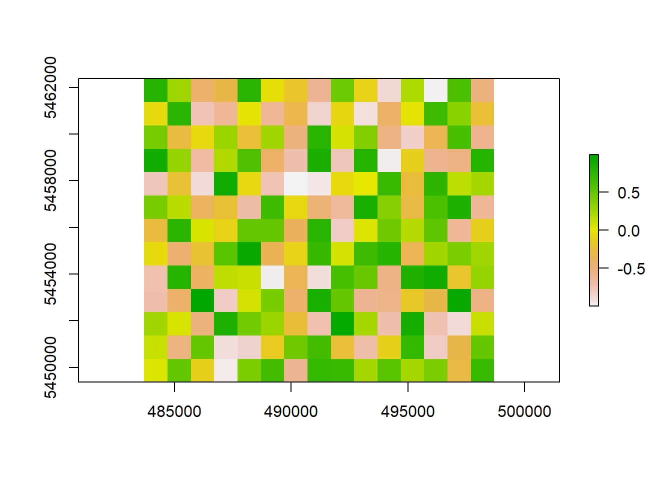
This map doesn’t exhibits complete spatial randomness, there is no pattern here! Which makes sense since we purposely created random data.
3.3 Read Spatial Data
Here we will only cover reading in tabular data with coordinates as point data, and ESRI shapefiles as these are very commonly available formats. For more details on the range of spatial data types in the wild I highly recommend Chapter 7 from the book Geocomputation with R.
3.3.1 Tabular Data with XY Coordinates
We often come across data that are in a tabular format such as .csv file where each row represents a specific event, and columns represent the characteristics of that event, including it’s latitude and longitude (i.e. the location). We want to take that a-spatial data format and convert it into one that we can map. In R, this becomes a fairly simple process which we will illustrate below using the ICBC data that can be downloaded in section 1.
First step is to read in the tabular data using the function read_csv() from the package readr.
icbc_crash <- read_csv("D:/Github/crash-course-gis-r/data/ICBC_cyclist_crashes.csv") # use the file location of where you have stored your data##
## -- Column specification ------------------------------------------------------------------------------------------------------------------------------------------------------------------------
## cols(
## .default = col_character(),
## `Date Of Loss Year` = col_double(),
## `Crash Count` = col_double(),
## Latitude = col_double(),
## Longitude = col_double(),
## `Number of Records` = col_double()
## )
## i Use `spec()` for the full column specifications.str(icbc_crash)#look at data frame## spec_tbl_df[,27] [10,204 x 27] (S3: spec_tbl_df/tbl_df/tbl/data.frame)
## $ Crash Breakdown 2 : chr [1:10204] "LOWER MAINLAND" "VANCOUVER ISLAND" "LOWER MAINLAND" "VANCOUVER ISLAND" ...
## $ Date Of Loss Year : num [1:10204] 2016 2016 2019 2019 2019 ...
## $ Crash Severity : chr [1:10204] "CASUALTY" "PROPERTY DAMAGE ONLY" "PROPERTY DAMAGE ONLY" "PROPERTY DAMAGE ONLY" ...
## $ Cyclist Flag : chr [1:10204] "Yes" "Yes" "Yes" "Yes" ...
## $ Day Of Week : chr [1:10204] "WEDNESDAY" "SATURDAY" "SATURDAY" "MONDAY" ...
## $ Derived Crash Congifuration: chr [1:10204] "UNDETERMINED" "SINGLE VEHICLE" "UNDETERMINED" "SINGLE VEHICLE" ...
## $ Intersection Crash : chr [1:10204] "Yes" "Yes" "Yes" "No" ...
## $ Month Of Year : chr [1:10204] "JULY" "NOVEMBER" "AUGUST" "AUGUST" ...
## $ Motorcycle Flag : chr [1:10204] "No" "No" "No" "No" ...
## $ Municipality Name (ifnull) : chr [1:10204] "ABBOTSFORD" "SOOKE" "SURREY" "VICTORIA" ...
## $ Parking Lot Flag : chr [1:10204] "No" "No" "No" "No" ...
## $ Pedestrian Flag : chr [1:10204] "No" "No" "No" "No" ...
## $ Region : chr [1:10204] "LOWER MAINLAND" "VANCOUVER ISLAND" "LOWER MAINLAND" "VANCOUVER ISLAND" ...
## $ Street Full Name (ifnull) : chr [1:10204] "MARSHALL RD" "CHURCH HILL DR" "24 AVE" "QUADRA ST" ...
## $ Time Category : chr [1:10204] "09:00-11:59" "15:00-17:59" "00:00-02:59" "15:00-17:59" ...
## $ Crash Breakdown : chr [1:10204] "WEDNESDAY" "SATURDAY" "SATURDAY" "MONDAY" ...
## $ Cross Street Full Name : chr [1:10204] "MCKENZIE RD" "STEEPLE CHASE" "KING GEORGE HWY" NA ...
## $ Heavy Veh Flag : chr [1:10204] "N" "N" "N" "N" ...
## $ Mid Block Crash : chr [1:10204] "N" "N" "N" "N" ...
## $ Municipality Name : chr [1:10204] "ABBOTSFORD" "SOOKE" "SURREY" "VICTORIA" ...
## $ Municipality With Boundary : chr [1:10204] "ABBOTSFORD" "SOOKE" "SURREY" "VICTORIA" ...
## $ Road Location Description : chr [1:10204] "MARSHALL RD & MCKENZIE RD" "CHURCH HILL DR & STEEPLE CHASE" "24 AVE & KING GEORGE BLVD & TURNING LANE" "QUADRA ST" ...
## $ Street Full Name : chr [1:10204] "MARSHALL RD" "CHURCH HILL DR" "24 AVE" "QUADRA ST" ...
## $ Crash Count : num [1:10204] 1 1 1 1 1 1 1 1 1 1 ...
## $ Latitude : num [1:10204] 49 48.4 49 48.4 48.4 ...
## $ Longitude : num [1:10204] -122 -124 -123 -123 -123 ...
## $ Number of Records : num [1:10204] 1 1 1 1 1 1 1 1 1 1 ...
## - attr(*, "spec")=
## .. cols(
## .. `Crash Breakdown 2` = col_character(),
## .. `Date Of Loss Year` = col_double(),
## .. `Crash Severity` = col_character(),
## .. `Cyclist Flag` = col_character(),
## .. `Day Of Week` = col_character(),
## .. `Derived Crash Congifuration` = col_character(),
## .. `Intersection Crash` = col_character(),
## .. `Month Of Year` = col_character(),
## .. `Motorcycle Flag` = col_character(),
## .. `Municipality Name (ifnull)` = col_character(),
## .. `Parking Lot Flag` = col_character(),
## .. `Pedestrian Flag` = col_character(),
## .. Region = col_character(),
## .. `Street Full Name (ifnull)` = col_character(),
## .. `Time Category` = col_character(),
## .. `Crash Breakdown` = col_character(),
## .. `Cross Street Full Name` = col_character(),
## .. `Heavy Veh Flag` = col_character(),
## .. `Mid Block Crash` = col_character(),
## .. `Municipality Name` = col_character(),
## .. `Municipality With Boundary` = col_character(),
## .. `Road Location Description` = col_character(),
## .. `Street Full Name` = col_character(),
## .. `Crash Count` = col_double(),
## .. Latitude = col_double(),
## .. Longitude = col_double(),
## .. `Number of Records` = col_double()
## .. )We can see there are two columns Latitude and Longitude corresponding to the location of each crash. Let’s check to see if there are missing values the records that have NA values for locations, and remove them.
is.na(icbc_crash$Latitude) %>% summary() #check for missing values in latitude## Mode FALSE TRUE
## logical 8673 1531is.na(icbc_crash$Longitude) %>% summary() #check for missing values in longitude## Mode FALSE TRUE
## logical 8673 1531icbc_crash <- icbc_crash %>%
filter(!is.na(Latitude)) # remove the records which have missing values
is.na(icbc_crash$Latitude) %>% summary()## Mode FALSE
## logical 8673is.na(icbc_crash$Longitude) %>% summary()## Mode FALSE
## logical 8673The next step is to use the st_as_sf() function from the sf package. We need to supply three inputs into the function: 1) the data frame and 2) the column names representing longitude and latitude coordinates as an R vector and 3) the coordinate system information. Remember that longitude represents locations from East to West which is equivalent to the X-axis values, and latitude represents values from North to South which is equivalent to the Y-axis. Make sure to check the data source for information on which specific geographic coordinate system the latitude and longitude represent. If this information is not available, it generally a safe bet to assume its WGS1984.
icbc_crash_sf <- st_as_sf(icbc_crash, coords = c("Longitude","Latitude"), crs = 4326)

str(icbc_crash_sf)
## sf[,26] [8,673 x 26] (S3: sf/tbl_df/tbl/data.frame)
## $ Crash Breakdown 2 : chr [1:8673] "LOWER MAINLAND" "VANCOUVER ISLAND" "LOWER MAINLAND" "VANCOUVER ISLAND" ...
## $ Date Of Loss Year : num [1:8673] 2016 2016 2019 2019 2019 ...
## $ Crash Severity : chr [1:8673] "CASUALTY" "PROPERTY DAMAGE ONLY" "PROPERTY DAMAGE ONLY" "PROPERTY DAMAGE ONLY" ...
## $ Cyclist Flag : chr [1:8673] "Yes" "Yes" "Yes" "Yes" ...
## $ Day Of Week : chr [1:8673] "WEDNESDAY" "SATURDAY" "SATURDAY" "MONDAY" ...
## $ Derived Crash Congifuration: chr [1:8673] "UNDETERMINED" "SINGLE VEHICLE" "UNDETERMINED" "SINGLE VEHICLE" ...
## $ Intersection Crash : chr [1:8673] "Yes" "Yes" "Yes" "No" ...
## $ Month Of Year : chr [1:8673] "JULY" "NOVEMBER" "AUGUST" "AUGUST" ...
## $ Motorcycle Flag : chr [1:8673] "No" "No" "No" "No" ...
## $ Municipality Name (ifnull) : chr [1:8673] "ABBOTSFORD" "SOOKE" "SURREY" "VICTORIA" ...
## $ Parking Lot Flag : chr [1:8673] "No" "No" "No" "No" ...
## $ Pedestrian Flag : chr [1:8673] "No" "No" "No" "No" ...
## $ Region : chr [1:8673] "LOWER MAINLAND" "VANCOUVER ISLAND" "LOWER MAINLAND" "VANCOUVER ISLAND" ...
## $ Street Full Name (ifnull) : chr [1:8673] "MARSHALL RD" "CHURCH HILL DR" "24 AVE" "QUADRA ST" ...
## $ Time Category : chr [1:8673] "09:00-11:59" "15:00-17:59" "00:00-02:59" "15:00-17:59" ...
## $ Crash Breakdown : chr [1:8673] "WEDNESDAY" "SATURDAY" "SATURDAY" "MONDAY" ...
## $ Cross Street Full Name : chr [1:8673] "MCKENZIE RD" "STEEPLE CHASE" "KING GEORGE HWY" NA ...
## $ Heavy Veh Flag : chr [1:8673] "N" "N" "N" "N" ...
## $ Mid Block Crash : chr [1:8673] "N" "N" "N" "N" ...
## $ Municipality Name : chr [1:8673] "ABBOTSFORD" "SOOKE" "SURREY" "VICTORIA" ...
## $ Municipality With Boundary : chr [1:8673] "ABBOTSFORD" "SOOKE" "SURREY" "VICTORIA" ...
## $ Road Location Description : chr [1:8673] "MARSHALL RD & MCKENZIE RD" "CHURCH HILL DR & STEEPLE CHASE" "24 AVE & KING GEORGE BLVD & TURNING LANE" "QUADRA ST" ...
## $ Street Full Name : chr [1:8673] "MARSHALL RD" "CHURCH HILL DR" "24 AVE" "QUADRA ST" ...
## $ Crash Count : num [1:8673] 1 1 1 1 1 1 1 1 1 1 ...
## $ Number of Records : num [1:8673] 1 1 1 1 1 1 1 1 1 1 ...
## $ geometry :sfc_POINT of length 8673; first list element: 'XY' num [1:2] -122 49
## - attr(*, "sf_column")= chr "geometry"
## - attr(*, "agr")= Factor w/ 3 levels "constant","aggregate",..: NA NA NA NA NA NA NA NA NA NA ...
## ..- attr(*, "names")= chr [1:25] "Crash Breakdown 2" "Date Of Loss Year" "Crash Severity" "Cyclist Flag" ...plot(icbc_crash_sf["Cyclist Flag"])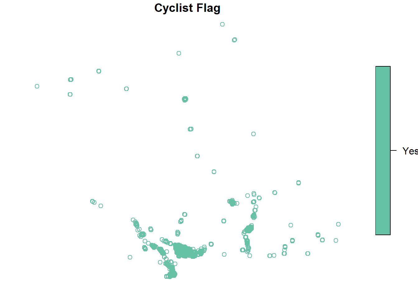
Finally, we can then convert these data into a projected coordinate system. You will need to “project” the data if you want to perform spatial operations on them (like we will do next chapter). We will use the function suggest_crs from the package crsuggest to attempt to figure out the right one for our data
possible_crs <- suggest_crs(icbc_crash_sf,units = "m",limit = 20)

possible_crs #View the the top 10 suggestions
## # A tibble: 20 x 6
## crs_code crs_name crs_type crs_gcs crs_units crs_proj4
## <chr> <chr> <chr> <dbl> <chr> <chr>
## 1 6596 NAD83(2011) / Washington North project~ 6318 m +proj=lcc +lat_0=47 +lon_0=-120.833333333333 +lat_1=48.7333333333333 +lat_2=47.5 +x_0=500000 +y_0=0 +ellps=GRS80 +uni~
## 2 3689 NAD83(NSRS2007) / Washington North project~ 4759 m +proj=lcc +lat_0=47 +lon_0=-120.833333333333 +lat_1=48.7333333333333 +lat_2=47.5 +x_0=500000 +y_0=0 +ellps=GRS80 +tow~
## 3 32148 NAD83 / Washington North project~ 4269 m +proj=lcc +lat_0=47 +lon_0=-120.833333333333 +lat_1=48.7333333333333 +lat_2=47.5 +x_0=500000 +y_0=0 +datum=NAD83 +uni~
## 4 2855 NAD83(HARN) / Washington North project~ 4152 m +proj=lcc +lat_0=47 +lon_0=-120.833333333333 +lat_1=48.7333333333333 +lat_2=47.5 +x_0=500000 +y_0=0 +ellps=GRS80 +tow~
## 5 3802 NAD83(CSRS) / Alberta 3TM ref mer~ project~ 4617 m +proj=tmerc +lat_0=0 +lon_0=-120 +k=0.9999 +x_0=0 +y_0=0 +ellps=GRS80 +towgs84=0,0,0,0,0,0,0 +units=m +no_defs
## 6 3801 NAD83 / Alberta 3TM ref merid 120~ project~ 4269 m +proj=tmerc +lat_0=0 +lon_0=-120 +k=0.9999 +x_0=0 +y_0=0 +datum=NAD83 +units=m +no_defs
## 7 3800 NAD27 / Alberta 3TM ref merid 120~ project~ 4267 m +proj=tmerc +lat_0=0 +lon_0=-120 +k=0.9999 +x_0=0 +y_0=0 +datum=NAD27 +units=m +no_defs
## 8 3403 NAD83(CSRS) / Alberta 10-TM (Reso~ project~ 4617 m +proj=tmerc +lat_0=0 +lon_0=-115 +k=0.9992 +x_0=0 +y_0=0 +ellps=GRS80 +towgs84=0,0,0,0,0,0,0 +units=m +no_defs
## 9 3402 NAD83(CSRS) / Alberta 10-TM (Fore~ project~ 4617 m +proj=tmerc +lat_0=0 +lon_0=-115 +k=0.9992 +x_0=500000 +y_0=0 +ellps=GRS80 +towgs84=0,0,0,0,0,0,0 +units=m +no_defs
## 10 3401 NAD83 / Alberta 10-TM (Resource) project~ 4269 m +proj=tmerc +lat_0=0 +lon_0=-115 +k=0.9992 +x_0=0 +y_0=0 +datum=NAD83 +units=m +no_defs
## 11 3400 NAD83 / Alberta 10-TM (Forest) project~ 4269 m +proj=tmerc +lat_0=0 +lon_0=-115 +k=0.9992 +x_0=500000 +y_0=0 +datum=NAD83 +units=m +no_defs
## 12 3153 NAD83(CSRS) / BC Albers project~ 4617 m +proj=aea +lat_0=45 +lon_0=-126 +lat_1=50 +lat_2=58.5 +x_0=1000000 +y_0=0 +ellps=GRS80 +towgs84=0,0,0,0,0,0,0 +units=~
## 13 3005 NAD83 / BC Albers project~ 4269 m +proj=aea +lat_0=45 +lon_0=-126 +lat_1=50 +lat_2=58.5 +x_0=1000000 +y_0=0 +datum=NAD83 +units=m +no_defs
## 14 3781 NAD83(CSRS) / Alberta 3TM ref mer~ project~ 4617 m +proj=tmerc +lat_0=0 +lon_0=-117 +k=0.9999 +x_0=0 +y_0=0 +ellps=GRS80 +towgs84=0,0,0,0,0,0,0 +units=m +no_defs
## 15 3777 NAD83 / Alberta 3TM ref merid 117~ project~ 4269 m +proj=tmerc +lat_0=0 +lon_0=-117 +k=0.9999 +x_0=0 +y_0=0 +datum=NAD83 +units=m +no_defs
## 16 3773 NAD27 / Alberta 3TM ref merid 117~ project~ 4267 m +proj=tmerc +lat_0=0 +lon_0=-117 +k=0.9999 +x_0=0 +y_0=0 +datum=NAD27 +units=m +no_defs
## 17 3740 NAD83(HARN) / UTM zone 10N project~ 4152 m +proj=utm +zone=10 +ellps=GRS80 +towgs84=0,0,0,0,0,0,0 +units=m +no_defs
## 18 26709 NAD27 / UTM zone 9N project~ 4267 m +proj=utm +zone=9 +datum=NAD27 +units=m +no_defs
## 19 3741 NAD83(HARN) / UTM zone 11N project~ 4152 m +proj=utm +zone=11 +ellps=GRS80 +towgs84=0,0,0,0,0,0,0 +units=m +no_defs
## 20 6340 NAD83(2011) / UTM zone 11N project~ 6318 m +proj=utm +zone=11 +ellps=GRS80 +units=m +no_defsThe suggest_crs() function return the top 10 matches for our dataset. To be clear, one should not blindly rely on this package to pick a projection for the data It is important to marry the convenience of suggest_crs with some research on what will work for the dataset. Particularly since, most of these suggestions are not good projections for mapping data for the entire province of British Columbia. I would think of this function as a handy way to list potential projections and the EPSG codes that one can cross reference with your own search on the internet for confirmation. It just so happens that the The BC Albers projection is the recommended map projection for analysis of the entire province.
Once we select a projection we can easily “transform” our data into that coordinate system using the function st_transform() and specifying the EPSG code associated with that coordinate system. We can check the CRS information of an sf object using the function st_crs().
icbc_crash_sf_proj <- st_transform(icbc_crash_sf,crs=3005)

st_crs(icbc_crash_sf_proj)
## Coordinate Reference System:
## User input: EPSG:3005
## wkt:
## PROJCRS["NAD83 / BC Albers",
## BASEGEOGCRS["NAD83",
## DATUM["North American Datum 1983",
## ELLIPSOID["GRS 1980",6378137,298.257222101,
## LENGTHUNIT["metre",1]]],
## PRIMEM["Greenwich",0,
## ANGLEUNIT["degree",0.0174532925199433]],
## ID["EPSG",4269]],
## CONVERSION["British Columbia Albers",
## METHOD["Albers Equal Area",
## ID["EPSG",9822]],
## PARAMETER["Latitude of false origin",45,
## ANGLEUNIT["degree",0.0174532925199433],
## ID["EPSG",8821]],
## PARAMETER["Longitude of false origin",-126,
## ANGLEUNIT["degree",0.0174532925199433],
## ID["EPSG",8822]],
## PARAMETER["Latitude of 1st standard parallel",50,
## ANGLEUNIT["degree",0.0174532925199433],
## ID["EPSG",8823]],
## PARAMETER["Latitude of 2nd standard parallel",58.5,
## ANGLEUNIT["degree",0.0174532925199433],
## ID["EPSG",8824]],
## PARAMETER["Easting at false origin",1000000,
## LENGTHUNIT["metre",1],
## ID["EPSG",8826]],
## PARAMETER["Northing at false origin",0,
## LENGTHUNIT["metre",1],
## ID["EPSG",8827]]],
## CS[Cartesian,2],
## AXIS["(E)",east,
## ORDER[1],
## LENGTHUNIT["metre",1]],
## AXIS["(N)",north,
## ORDER[2],
## LENGTHUNIT["metre",1]],
## USAGE[
## SCOPE["Province-wide spatial data management."],
## AREA["Canada - British Columbia."],
## BBOX[48.25,-139.04,60.01,-114.08]],
## ID["EPSG",3005]]But let’s say that we only wanted to map data in Vancouver. What map projection would we use then? We can isolate only the records in Vancouver using data query based on the column Municipality Name. This is a short preview of what we call “attribute queries” in the GIS world and we will get into this more in the next chapter. But for now just know that we use the filter() function to select specific geographic features (in this case points) where the "Municipality Name" is “VANCOUVER.” We can then use the suggest_crs() function again here and see what are the suggested projections for mapping data at a more local level.
icbc_crash_van <- icbc_crash_sf %>%
  filter(`Municipality Name`=="VANCOUVER")

plot(icbc_crash_van["Cyclist Flag"])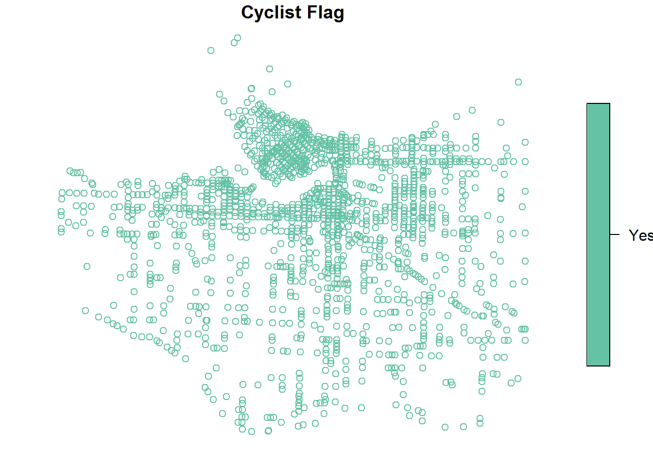
possible_crs_van <- suggest_crs(icbc_crash_van)

possible_crs_van
## # A tibble: 10 x 6
## crs_code crs_name crs_type crs_gcs crs_units crs_proj4
## <chr> <chr> <chr> <dbl> <chr> <chr>
## 1 3153 NAD83(CSRS) / BC Albers projected 4617 m +proj=aea +lat_0=45 +lon_0=-126 +lat_1=50 +lat_2=58.5 +x_0=1000000 +y_0=0 +ellps=GRS80 +towgs84=0,0,0,0,0,0,0 +units=~
## 2 3005 NAD83 / BC Albers projected 4269 m +proj=aea +lat_0=45 +lon_0=-126 +lat_1=50 +lat_2=58.5 +x_0=1000000 +y_0=0 +datum=NAD83 +units=m +no_defs
## 3 26710 NAD27 / UTM zone 10N projected 4267 m +proj=utm +zone=10 +datum=NAD27 +units=m +no_defs
## 4 3157 NAD83(CSRS) / UTM zone 10N projected 4617 m +proj=utm +zone=10 +ellps=GRS80 +towgs84=0,0,0,0,0,0,0 +units=m +no_defs
## 5 26910 NAD83 / UTM zone 10N projected 4269 m +proj=utm +zone=10 +datum=NAD83 +units=m +no_defs
## 6 32610 WGS 84 / UTM zone 10N projected 4326 m +proj=utm +zone=10 +datum=WGS84 +units=m +no_defs
## 7 32410 WGS 72BE / UTM zone 10N projected 4324 m +proj=utm +zone=10 +ellps=WGS72 +towgs84=0,0,1.9,0,0,0.814,-0.38 +units=m +no_defs
## 8 32210 WGS 72 / UTM zone 10N projected 4322 m +proj=utm +zone=10 +ellps=WGS72 +towgs84=0,0,4.5,0,0,0.554,0.2263 +units=m +no_defs
## 9 3979 NAD83(CSRS) / Canada Atlas Lambe~ projected 4617 m +proj=lcc +lat_0=49 +lon_0=-95 +lat_1=49 +lat_2=77 +x_0=0 +y_0=0 +ellps=GRS80 +towgs84=0,0,0,0,0,0,0 +units=m +no_defs
## 10 3978 NAD83 / Canada Atlas Lambert projected 4269 m +proj=lcc +lat_0=49 +lon_0=-95 +lat_1=49 +lat_2=77 +x_0=0 +y_0=0 +datum=NAD83 +units=m +no_defsIn the case of data at a local/regional scale (E.g. a town or city), it is almost always a good choice to use a UTM projection. The UTM projection divides the earth into 60 zones from east to west (e.g. 3.2).
](images/utm.png)
Figure 3.2: UTM Zones across Northern Mexico, the United States and sourthern CanadaSource
Distortion within a UTM zone is minimized, while outside of it it is very distorted. The appropriate UTM projection here is UTM Zone 10N which is amongst the suggested CRS’s. We will select NAD83 / UTM zone 10N and transform it into this projection.
icbc_crash_van_proj <- st_transform(icbc_crash_van,crs=26910)

plot(icbc_crash_van_proj["Cyclist Flag"])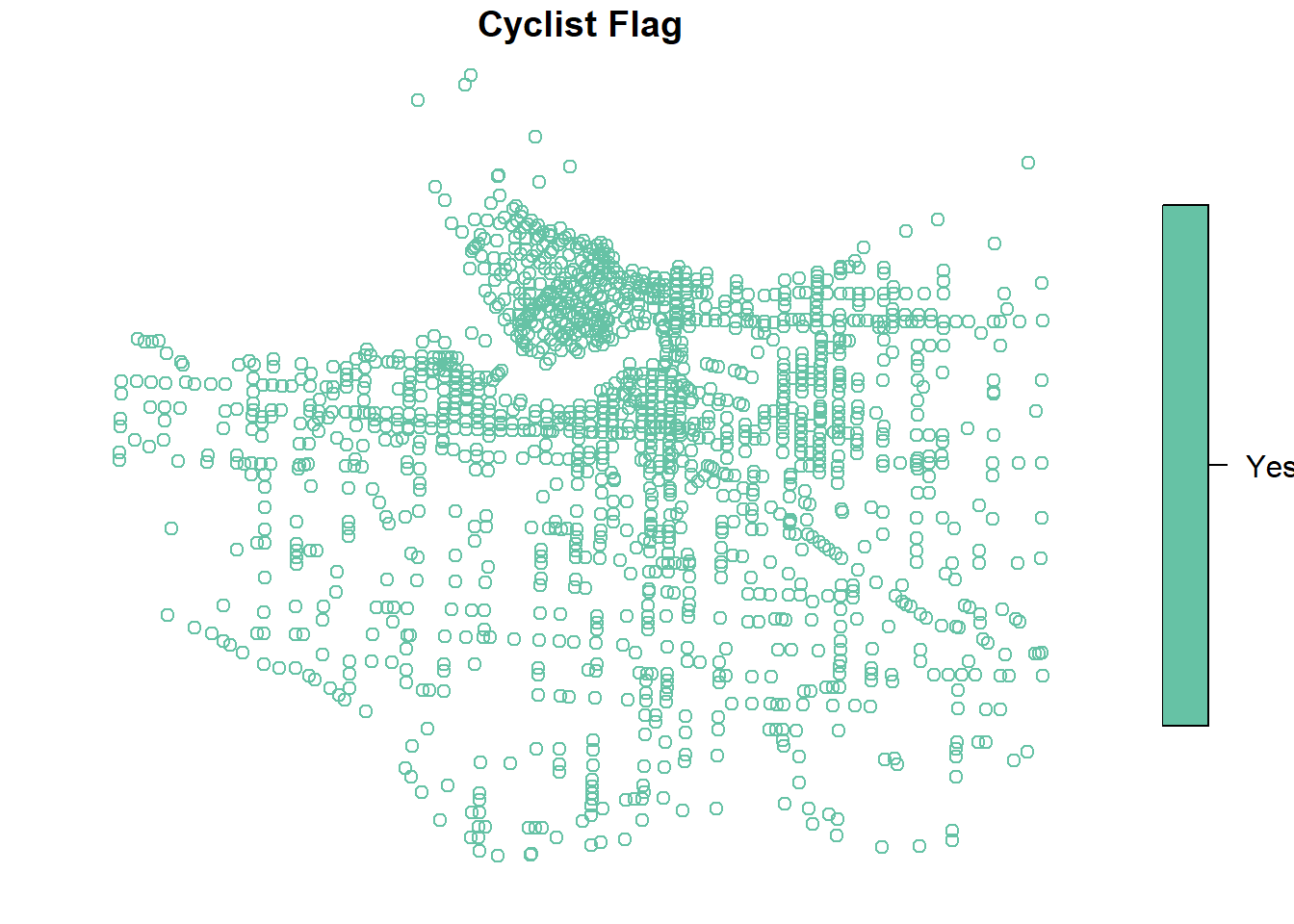
3.3.2 Shapefiles
Shapefiles are a data format for storing vector data that is proprietary to a company called ESRI which produces the very popular, and widely used ArcGIS products. You will often come across these files in your day to day work. A shapefile is actually a collection of several different kinds of files that store different information. These include a .shp, .shx, .dbf and .prj files among other (see https://en.wikipedia.org/wiki/Shapefile for a good description). It isn’t important right now to know what each file means, but know that they work together to represent a spatial data object within a GIS so make sure that you keep al the seemingly random files together if moving them from place to place, not just the .shp file. In R it is easy to import a shapefile using the read_sf() function from the sf package. We will load a polygon shapefile called CoV_Boundary that was included in the data download from Chapter 1.
Figure 3.3: Example Shapefile
As you can see this shapefile consists of multiple files. When loading a shapefile always point to the .shp file as done below. read_sf() will load the information from the other files automatically including the attribute data (.dbf), the coordinate system infomration (.prj) and the geometry information (.shp and .shx) and combine them directly into an sf object.
van_boundary <- read_sf("D:/Github/crash-course-gis-r/data/CoV_boundary.shp") # use the file location of where you have stored your data
van_boundary
## Simple feature collection with 1 feature and 11 fields
## Geometry type: POLYGON
## Dimension: XY
## Bounding box: xmin: 483610.9 ymin: 5449455 xmax: 498409.2 ymax: 5462461
## Projected CRS: NAD83 / UTM zone 10N
## # A tibble: 1 x 12
## Popultn Hoshlds GeoUID Type PR_UID ShapeAr Dwllngs name AP_Cns_ CD_UID CMA_UID geometry
## <int> <int> <chr> <chr> <chr> <dbl> <int> <chr> <int> <chr> <chr> <POLYGON [m]>
## 1 631486 283916 5915022 CSD 59 116. 309418 Vancouver (CY) 603502 5915 59933 ((489370.1 5458479, 489445.3 5458536, 489448.6 5458539, 489452.1 5458541, 489455.7 545854...plot(van_boundary["Type"])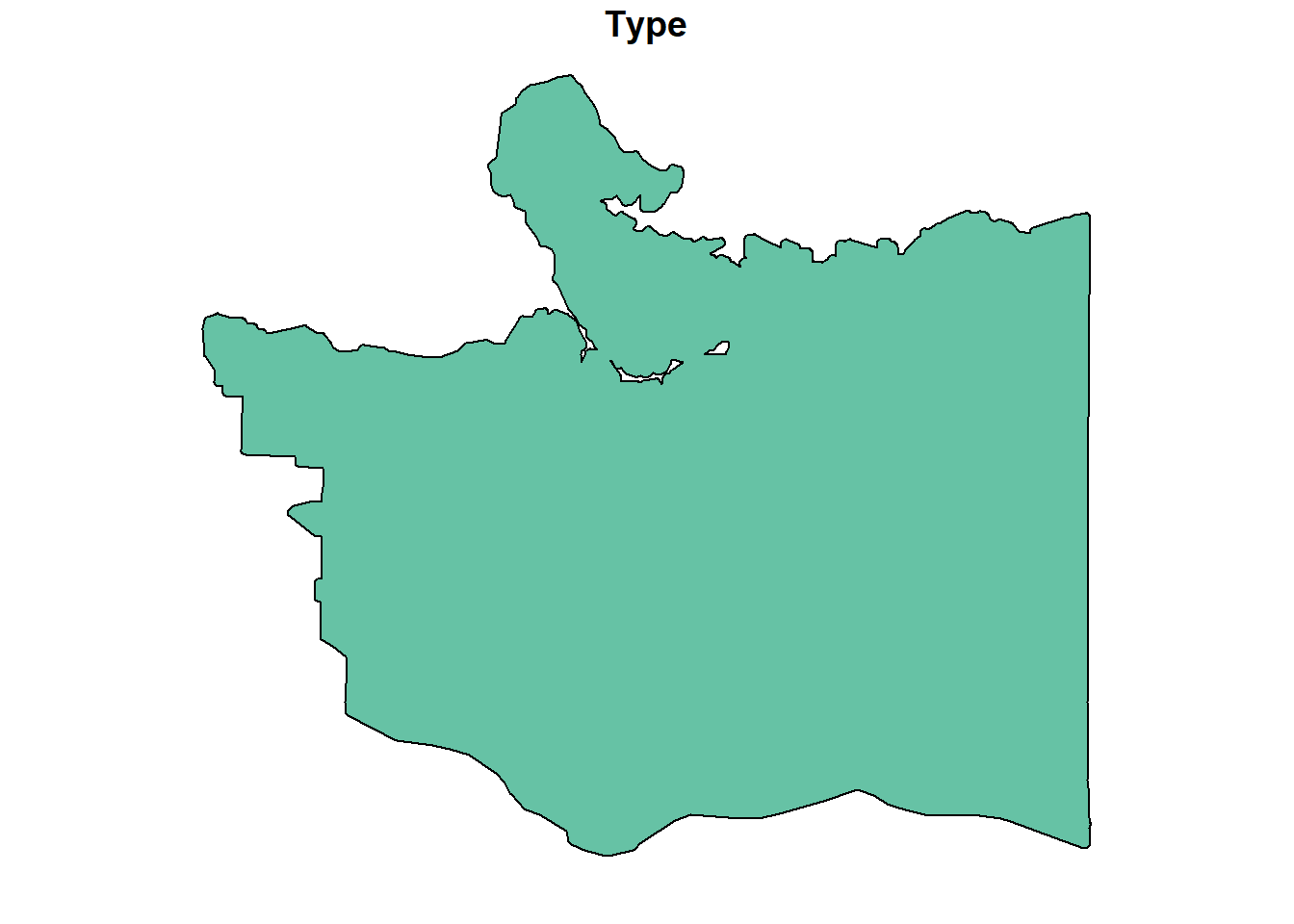 We can see that this shapefile is already in a projected coordinate system, and consists of 1 polygon with some population characteristics.
3.3.3 Programmatically
In the past collecting GIS data involved going to a bunch of different websites and manually downloading the data you needed and trying to organize it within your hard drive, and loading each dataset into the GIS from there. Nowadays it is becoming increasingly easy to programmatically access spatial data (and non-spatial) using packages that are specifically designed to enable you retrieve data from specific places. Here we will go through two such packages. With these packages there is no need to manually download data from sites and save to your computer, you can just load it directly from R using their provided code! These include:
osmdata: retrieve various built environment data from OpenStreetMapscancensus: retrieve national census data aggregated to census geographies from Statistics Canada
3.3.3.1 OpenStreetMaps
The osmdata package can be used to download OpenStreetMaps data. OpenStreetMap is a database of crowdsourced geographic information that includes things like road networks, water features, points of itnerest and more. Whatever a person on the internet can map and has mapped on OSM is available for download for free. For a more detailed introduction with more exploration of the functionality of the package I point you towards the very helpful vignette. Here we will simply download the street network information for the City of Vancouver to get you started.
First we need to define the study area from which to retrieve data using the function getbb(). This function takes a string and returns a rectangular bounding box for the area of interest.
van_bb <- getbb("Vancouver BC")

van_bb
## min max
## x -123.22496 -123.02324
## y 49.19845 49.31617Next we input the bounding box we just retrieved into the opq() function to query OSM data and combine with add_osm_feature() function to obtain open street map road network data. We use the character key “highway” to specify we are interested int the road network data. Other types of data we can obtain can be found here: https://wiki.openstreetmap.org/wiki/. We then use the function osmdata_sf() to convert the query into a spatial sf object.
#define
opq_van <- opq(bbox = van_bb)

osm_van <- add_osm_feature(opq = opq_van,
                          key = "highway"
                           )

osm_van_sf <- osmdata_sf(osm_van)

osm_van_sf
## Object of class 'osmdata' with:
## $bbox : 49.1984452,-123.2249611,49.3161714,-123.0232419
## $overpass_call : The call submitted to the overpass API
## $meta : metadata including timestamp and version numbers
## $osm_points : 'sf' Simple Features Collection with 143518 points
## $osm_lines : 'sf' Simple Features Collection with 33125 linestrings
## $osm_polygons : 'sf' Simple Features Collection with 4074 polygons
## $osm_multilines : NULL
## $osm_multipolygons : 'sf' Simple Features Collection with 21 multipolygonsWe now have a data object of class osmdata. We can’t work directly with this data yet. To obtain the street network spatial data specifically we need to retrieve one part of the osmdata object called osm_lines using the $ operator.
osm_van_network <- osm_van_sf$osm_lines

osm_van_network
## Simple feature collection with 33125 features and 235 fields
## Geometry type: LINESTRING
## Dimension: XY
## Bounding box: xmin: -123.2623 ymin: 49.18012 xmax: -122.981 ymax: 49.33017
## Geodetic CRS: WGS 84
## First 10 features:
## osm_id name Note2 access addr.city addr.housenumber addr.postcode addr.street alt_name amenity area area.highway attribution barrier bicycle boundary bridge
## 4231647 4231647 West King Edward Avenue <NA> <NA> <NA> <NA> <NA> <NA> <NA> <NA> <NA> <NA> <NA> <NA> <NA> <NA> <NA>
## 4231648 4231648 Granville Street <NA> <NA> <NA> <NA> <NA> <NA> <NA> <NA> <NA> <NA> <NA> <NA> <NA> <NA> <NA>
## 4231651 4231651 East 12th Avenue <NA> <NA> <NA> <NA> <NA> <NA> <NA> <NA> <NA> <NA> <NA> <NA> <NA> <NA> <NA>
## 4231652 4231652 South Grandview Highway <NA> <NA> <NA> <NA> <NA> <NA> <NA> <NA> <NA> <NA> <NA> <NA> <NA> <NA> <NA>
## bridge.colour bridge.name bridge.structure bridge.type bridge_name bridge_name.en bridge_name.fr building building.levels bus bus.lanes bus_bay busway button_operated canvec.CODE
## 4231647 <NA> <NA> <NA> <NA> <NA> <NA> <NA> <NA> <NA> <NA> <NA> <NA> <NA> <NA> <NA>
## 4231648 <NA> <NA> <NA> <NA> <NA> <NA> <NA> <NA> <NA> <NA> <NA> <NA> <NA> <NA> <NA>
## 4231651 <NA> <NA> <NA> <NA> <NA> <NA> <NA> <NA> <NA> <NA> <NA> <NA> <NA> <NA> <NA>
## 4231652 <NA> <NA> <NA> <NA> <NA> <NA> <NA> <NA> <NA> <NA> <NA> <NA> <NA> <NA> <NA>
## car change.lanes.backward change.lanes.forward check_date comment construction conveying covered created_by crossing crossing.island cutting cycleway cycleway.both cycleway.both.lane
## 4231647 <NA> <NA> <NA> <NA> <NA> <NA> <NA> <NA> <NA> <NA> <NA> <NA> <NA> <NA> <NA>
## 4231648 <NA> <NA> <NA> <NA> <NA> <NA> <NA> <NA> <NA> <NA> <NA> <NA> <NA> <NA> <NA>
## 4231651 <NA> <NA> <NA> <NA> <NA> <NA> <NA> <NA> <NA> <NA> <NA> <NA> <NA> <NA> <NA>
## 4231652 <NA> <NA> <NA> <NA> <NA> <NA> <NA> <NA> <NA> <NA> <NA> <NA> <NA> <NA> <NA>
## cycleway.left cycleway.right cycleway.right.lane cycleway.surface description description.bicycle destination destination.backward destination.forward destination.lanes
## 4231647 <NA> lane <NA> <NA> <NA> <NA> <NA> <NA> <NA> <NA>
## 4231648 <NA> <NA> <NA> <NA> <NA> <NA> <NA> <NA> <NA> <NA>
## 4231651 <NA> <NA> <NA> <NA> <NA> <NA> <NA> <NA> <NA> <NA>
## 4231652 <NA> <NA> <NA> <NA> <NA> <NA> <NA> <NA> <NA> <NA>
## destination.ref destination.ref.lanes destination.ref.to destination.street destination.symbol direction dog dogs embankment end_date est_width except fixme floating foot footway
## 4231647 <NA> <NA> <NA> <NA> <NA> <NA> <NA> <NA> <NA> <NA> <NA> <NA> <NA> <NA> <NA> <NA>
## 4231648 <NA> <NA> <NA> <NA> <NA> <NA> <NA> <NA> <NA> <NA> <NA> <NA> <NA> <NA> <NA> <NA>
## 4231651 <NA> <NA> <NA> <NA> <NA> <NA> <NA> <NA> <NA> <NA> <NA> <NA> <NA> <NA> <NA> <NA>
## 4231652 <NA> <NA> <NA> <NA> <NA> <NA> <NA> <NA> <NA> <NA> <NA> <NA> <NA> <NA> <NA> <NA>
## footway.surface geobase.acquisitionTechnique geobase.datasetName geobase.uuid golf golf_cart handrail hazmat height hgv highway historic horse hov.lanes hov.minimum incline indoor
## 4231647 <NA> <NA> <NA> <NA> <NA> <NA> <NA> <NA> <NA> <NA> secondary <NA> <NA> <NA> <NA> <NA> <NA>
## 4231648 <NA> <NA> <NA> <NA> <NA> <NA> <NA> <NA> <NA> <NA> trunk <NA> <NA> <NA> <NA> <NA> <NA>
## 4231651 <NA> <NA> <NA> <NA> <NA> <NA> <NA> <NA> <NA> no secondary <NA> <NA> <NA> <NA> <NA> <NA>
## 4231652 <NA> <NA> <NA> <NA> <NA> <NA> <NA> <NA> <NA> no secondary <NA> <NA> <NA> <NA> <NA> <NA>
## informal information internet_access internet_access.fee is_in junction junction.ref kerb landuse lane_markings lanes lanes.backward lanes.bus lanes.bus.backward
## 4231647 <NA> <NA> <NA> <NA> <NA> <NA> <NA> <NA> <NA> <NA> 1 <NA> <NA> <NA>
## 4231648 <NA> <NA> <NA> <NA> <NA> <NA> <NA> <NA> <NA> <NA> 6 <NA> <NA> <NA>
## 4231651 <NA> <NA> <NA> <NA> <NA> <NA> <NA> <NA> <NA> <NA> <NA> <NA> <NA> <NA>
## 4231652 <NA> <NA> <NA> <NA> <NA> <NA> <NA> <NA> <NA> <NA> <NA> <NA> <NA> <NA>
## lanes.bus.backward.conditional lanes.bus.conditional lanes.bus.forward lanes.bus.forward.conditional lanes.forward layer lcn lcn_ref leisure level line lit loc_name location
## 4231647 <NA> <NA> <NA> <NA> <NA> <NA> <NA> <NA> <NA> <NA> <NA> <NA> <NA> <NA>
## 4231648 <NA> <NA> <NA> <NA> <NA> <NA> <NA> <NA> <NA> <NA> <NA> <NA> <NA> <NA>
## 4231651 <NA> <NA> <NA> <NA> <NA> <NA> <NA> <NA> <NA> <NA> <NA> <NA> <NA> <NA>
## 4231652 <NA> <NA> <NA> <NA> <NA> <NA> <NA> <NA> <NA> <NA> <NA> <NA> <NA> <NA>
## man_made maxheight maxspeed maxspeed.advisory maxspeed.conditional maxspeed.type maxweight min_height motor_vehicle motor_vehicle.lanes motorcar motorcycle motorcycle.lanes mtb.scale
## 4231647 <NA> <NA> 50 <NA> <NA> <NA> <NA> <NA> <NA> <NA> <NA> <NA> <NA> <NA>
## 4231648 <NA> <NA> 50 <NA> <NA> <NA> <NA> <NA> <NA> <NA> <NA> <NA> <NA> <NA>
## 4231651 <NA> <NA> 50 <NA> <NA> <NA> <NA> <NA> <NA> <NA> <NA> <NA> <NA> <NA>
## 4231652 <NA> <NA> 50 <NA> <NA> <NA> <NA> <NA> <NA> <NA> <NA> <NA> <NA> <NA>
## name.en name.fr name.zh natural network noexit noname note note1 note.bicycle note_2 official_name old_railway_operator old_ref oneway oneway.bicycle opening_date opening_hours
## 4231647 <NA> <NA> <NA> <NA> <NA> <NA> <NA> <NA> <NA> <NA> <NA> <NA> <NA> <NA> yes <NA> <NA> <NA>
## 4231648 <NA> <NA> <NA> <NA> <NA> <NA> <NA> <NA> <NA> <NA> <NA> <NA> <NA> <NA> no <NA> <NA> <NA>
## 4231651 <NA> <NA> <NA> <NA> <NA> <NA> <NA> <NA> <NA> <NA> <NA> <NA> <NA> <NA> no <NA> <NA> <NA>
## 4231652 <NA> <NA> <NA> <NA> <NA> <NA> <NA> <NA> <NA> <NA> <NA> <NA> <NA> <NA> no <NA> <NA> <NA>
## operator parking.condition.both parking.condition.left parking.condition.left.time_interval parking.condition.right parking.lane.both parking.lane.left parking.lane.right phone pier
## 4231647 <NA> <NA> <NA> <NA> <NA> <NA> <NA> <NA> <NA> <NA>
## 4231648 <NA> <NA> <NA> <NA> <NA> <NA> <NA> <NA> <NA> <NA>
## 4231651 <NA> <NA> <NA> <NA> <NA> <NA> <NA> <NA> <NA> <NA>
## 4231652 <NA> <NA> <NA> <NA> <NA> <NA> <NA> <NA> <NA> <NA>
## place postal_code private psv public_transport railway ramp ramp_speed rcn_ref ref reg_name restriction rollerblades rollerblading roof.direction roof.height roof.shape route
## 4231647 <NA> <NA> <NA> <NA> <NA> <NA> <NA> <NA> <NA> <NA> <NA> <NA> <NA> <NA> <NA> <NA> <NA> <NA>
## 4231648 <NA> <NA> <NA> <NA> <NA> <NA> <NA> <NA> <NA> 99 <NA> <NA> <NA> <NA> <NA> <NA> <NA> <NA>
## 4231651 <NA> <NA> <NA> <NA> <NA> <NA> <NA> <NA> <NA> <NA> <NA> <NA> <NA> <NA> <NA> <NA> <NA> <NA>
## 4231652 <NA> <NA> <NA> <NA> <NA> <NA> <NA> <NA> <NA> <NA> <NA> <NA> <NA> <NA> <NA> <NA> <NA> <NA>
## sac_scale school_zone scooter seasonal segregated service shelter shop short_name shoulder sidewalk sidewalk.both.surface sidewalk.left sidewalk.left.surface sidewalk.left.width
## 4231647 <NA> <NA> <NA> <NA> <NA> <NA> <NA> <NA> <NA> <NA> <NA> <NA> <NA> <NA> <NA>
## 4231648 <NA> <NA> <NA> <NA> <NA> <NA> <NA> <NA> <NA> <NA> <NA> <NA> <NA> <NA> <NA>
## 4231651 <NA> <NA> <NA> <NA> <NA> <NA> <NA> <NA> <NA> <NA> <NA> <NA> <NA> <NA> <NA>
## 4231652 <NA> <NA> <NA> <NA> <NA> <NA> <NA> <NA> <NA> <NA> <NA> <NA> <NA> <NA> <NA>
## sidewalk.right skateboard smoothness source source1 source.bicycle source.bridge source.location source.maxspeed source.parking sport stairs start_date step_count stroller subway
## 4231647 <NA> <NA> <NA> <NA> <NA> <NA> <NA> <NA> <NA> <NA> <NA> <NA> <NA> <NA> <NA> <NA>
## 4231648 <NA> <NA> <NA> <NA> <NA> <NA> <NA> <NA> <NA> <NA> <NA> <NA> <NA> <NA> <NA> <NA>
## 4231651 <NA> <NA> <NA> <NA> <NA> <NA> <NA> <NA> <NA> <NA> <NA> <NA> <NA> <NA> <NA> <NA>
## 4231652 <NA> <NA> <NA> <NA> <NA> <NA> <NA> <NA> <NA> <NA> <NA> <NA> <NA> <NA> <NA> <NA>
## surface swimming_pool tactile_paving toilets tracktype traffic_calming traffic_signals trail_visibility transit.lanes trolley_wire trolleybus tunnel tunnel.name turn turn.lanes
## 4231647 asphalt <NA> <NA> <NA> <NA> <NA> <NA> <NA> <NA> <NA> <NA> <NA> <NA> <NA> <NA>
## 4231648 asphalt <NA> <NA> <NA> <NA> <NA> <NA> <NA> <NA> yes <NA> <NA> <NA> <NA> <NA>
## 4231651 asphalt <NA> <NA> <NA> <NA> <NA> <NA> <NA> <NA> <NA> <NA> <NA> <NA> <NA> <NA>
## 4231652 <NA> <NA> <NA> <NA> <NA> <NA> <NA> <NA> <NA> <NA> <NA> <NA> <NA> <NA> <NA>
## turn.lanes.backward turn.lanes.forward type url vehicle water website wheelchair width wikidata wikipedia geometry
## 4231647 <NA> <NA> <NA> <NA> <NA> <NA> <NA> <NA> <NA> <NA> <NA> LINESTRING (-123.1679 49.24...
## 4231648 <NA> <NA> <NA> <NA> <NA> <NA> <NA> <NA> <NA> <NA> <NA> LINESTRING (-123.1401 49.21...
## 4231651 <NA> <NA> <NA> <NA> <NA> <NA> <NA> <NA> <NA> <NA> <NA> LINESTRING (-123.0911 49.25...
## 4231652 <NA> <NA> <NA> <NA> <NA> <NA> <NA> <NA> <NA> <NA> <NA> LINESTRING (-123.0616 49.25...
## [ reached 'max' / getOption("max.print") -- omitted 6 rows ]We can see these from a quick glane at our street network data that they are unprojected. Lets project the dataset into UTM Zone 10, an appropriate map projection for Vancouver data. Then let’s quickly map the “highway” variable.
osm_van_network <- st_transform(osm_van_network,crs=26910) # project data

plot(osm_van_network["highway"],key.pos = 1)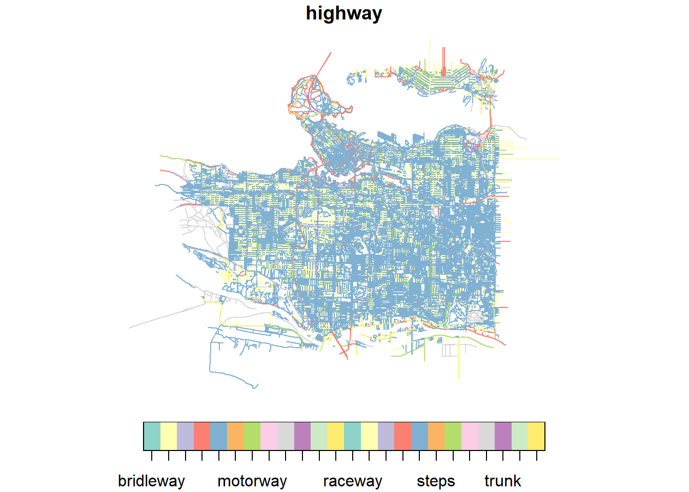
Now we have street network data ready to go from OSM! Pretty easy and a great way to get a consistent source of infrastructure data for your research, particularly in multi-city studies.
3.3.3.2 Canadian Census Geography
The cancensus package enables you to retrieve Canadian Census data programatically (i.e. downloading the data directly through R) including geographic data. The package allows you to retrieve data from 2006, 2011, and 2016 censuses. T
For future reference you can access a more detailed tutorial on using the cancensus package directly from the developer: https://mountainmath.github.io/cancensus/articles/cancensus.html. Here we will just get you started with downloading geographic data.
To start you will need to obtain a “CensusMapper API” key. Sign up for your API key here: https://censusmapper.ca/users/sign_up. Once you successfully make a profile and login, click on the top right button and click Edit Profile (see figure below).
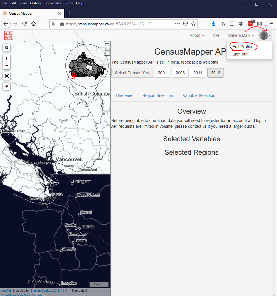
Figure 3.4: Screen shot of CensusMapper website
Once you successfully make a profile and login, click on the top right button and click Edit Profile. Your API key will be listed in this tab. Copy the API key to your clipboard for use in the next section.
options(cancensus.api_key = "your_api_key") # input your API Key here to enable retrieval of data from Statistics CanadaWe can access geographic census data through the function get_census(). To use this function we will need to find the specific area we want to download data for using the function list_census_regions(), as well as look up specific variables we are interested in using find_census_vectors(). Let’s retrieve Dissemination Area (DA) census geography for the City of Vancouver from the 2016 census with information on commute mode.
First let’s find the specific variables that we want:
find_census_vectors("Main mode of Commute",#search term
                    type = "total", # pick one of all, total, male or female in terms of counts
                    dataset = "CA16", #specify the 2016 census
                    query_type = "semantic"

                     )
## Multiple possible matches. Results ordered by closeness.## # A tibble: 7 x 4
## vector type label details
## <chr> <fct> <chr> <chr>
## 1 v_CA16_5~ Total Total - Main mode of commuting for the employed labour force aged 15 years and over~ 25% Data; Commute; Total - Main mode of commuting for the employed labour force aged 15 ~
## 2 v_CA16_5~ Total Car, truck, van - as a driver 25% Data; Commute; Total - Main mode of commuting for the employed labour force aged 15 ~
## 3 v_CA16_5~ Total Car, truck, van - as a passenger 25% Data; Commute; Total - Main mode of commuting for the employed labour force aged 15 ~
## 4 v_CA16_5~ Total Public transit 25% Data; Commute; Total - Main mode of commuting for the employed labour force aged 15 ~
## 5 v_CA16_5~ Total Walked 25% Data; Commute; Total - Main mode of commuting for the employed labour force aged 15 ~
## 6 v_CA16_5~ Total Bicycle 25% Data; Commute; Total - Main mode of commuting for the employed labour force aged 15 ~
## 7 v_CA16_5~ Total Other method 25% Data; Commute; Total - Main mode of commuting for the employed labour force aged 15 ~Second let’s find the identifying code for the study area:
list_census_regions("CA16")## Querying CensusMapper API for regions data...## # A tibble: 5,518 x 8
## region name level pop municipal_status CMA_UID CD_UID PR_UID
## <chr> <chr> <chr> <int> <chr> <chr> <chr> <chr>
## 1 01 Canada C 35151728 <NA> <NA> <NA> <NA>
## 2 35 Ontario PR 13448494 <NA> <NA> <NA> <NA>
## 3 24 Quebec PR 8164361 <NA> <NA> <NA> <NA>
## 4 59 British Columbia PR 4648055 <NA> <NA> <NA> <NA>
## 5 48 Alberta PR 4067175 <NA> <NA> <NA> <NA>
## 6 46 Manitoba PR 1278365 <NA> <NA> <NA> <NA>
## 7 47 Saskatchewan PR 1098352 <NA> <NA> <NA> <NA>
## 8 12 Nova Scotia PR 923598 <NA> <NA> <NA> <NA>
## 9 13 New Brunswick PR 747101 <NA> <NA> <NA> <NA>
## 10 10 Newfoundland and Labrador PR 519716 <NA> <NA> <NA> <NA>
## # ... with 5,508 more rowslist_census_regions("CA16") %>%
filter(name=="Vancouver") #isolate the census regions with the name "Vancouver"## Reading regions list from local cache.## # A tibble: 2 x 8
## region name level pop municipal_status CMA_UID CD_UID PR_UID
## <chr> <chr> <chr> <int> <chr> <chr> <chr> <chr>
## 1 59933 Vancouver CMA 2463431 B <NA> <NA> 59
## 2 5915022 Vancouver CSD 631486 CY 59933 5915 59There are two census areas named “Vancouver.” We are interested in the City of Vancouver which is represented by the region id of “5915022.” You can tell this is the case by examining the “level” variable which is CSD, standing for Census Subdivision as well as through the “municipal_status” variable which is CY standing for City.
Now let’s retrieve the geographic census data:
vancouver_da_2016 <- get_census(dataset='CA16', #specify the census of interest
                          regions=list(CSD="5915022"),#specify the region of interest
                          vectors=c("v_CA16_5792","v_CA16_5795","v_CA16_5798","
                                    v_CA16_5801","v_CA16_5804","v_CA16_5807",
                                    "v_CA16_5810"), # specify the attribute data of interest
                         labels = "short",# here we specify short variabhle names, otherwise they get very long
                           level='DA', #specify the census geography
                          geo_format = "sf",#specify the geographic data format as output
                         quiet = TRUE #turn off download progress messages (set to FALSE to see messages)

                          )


vancouver_da_2016
## Simple feature collection with 993 features and 18 fields
## Geometry type: MULTIPOLYGON
## Dimension: XY
## Bounding box: xmin: -123.2242 ymin: 49.19853 xmax: -123.0229 ymax: 49.31408
## Geodetic CRS: WGS 84
## First 10 features:
## Population Households GeoUID Type CD_UID Shape Area Dwellings CSD_UID CT_UID CMA_UID Region Name Area (sq km) v_CA16_5792 v_CA16_5795 v_CA16_5798 v_CA16_5804 v_CA16_5807 v_CA16_5810
## 1 632 254 59150307 DA 5915 0.29926 273 5915022 9330053.02 59933 Vancouver 0.29926 340 240 15 10 15 10
## 2 501 203 59150308 DA 5915 0.10956 223 5915022 9330053.02 59933 Vancouver 0.10956 260 165 0 15 20 10
## 3 745 269 59150309 DA 5915 0.11190 299 5915022 9330053.02 59933 Vancouver 0.11190 420 240 10 10 10 0
## 4 536 283 59150310 DA 5915 0.10940 310 5915022 9330053.02 59933 Vancouver 0.10940 230 130 0 15 10 0
## 5 532 181 59150311 DA 5915 0.08094 199 5915022 9330053.02 59933 Vancouver 0.08094 330 210 10 20 10 10
## 6 562 203 59150312 DA 5915 0.08706 211 5915022 9330053.02 59933 Vancouver 0.08706 310 170 10 10 10 0
## 7 1088 402 59150313 DA 5915 0.17284 418 5915022 9330052.02 59933 Vancouver 0.17284 415 280 20 0 20 10
## 8 556 170 59150328 DA 5915 0.23224 181 5915022 9330052.02 59933 Vancouver 0.23224 355 195 20 0 0 0
## 9 959 333 59150329 DA 5915 0.30854 356 5915022 9330052.02 59933 Vancouver 0.30854 435 275 15 25 10 0
## 10 506 174 59150330 DA 5915 0.07820 189 5915022 9330052.02 59933 Vancouver 0.07820 245 210 0 10 0 0
## geometry
## 1 MULTIPOLYGON (((-123.0233 4...
## 2 MULTIPOLYGON (((-123.0234 4...
## 3 MULTIPOLYGON (((-123.0283 4...
## 4 MULTIPOLYGON (((-123.0234 4...
## 5 MULTIPOLYGON (((-123.0257 4...
## 6 MULTIPOLYGON (((-123.0234 4...
## 7 MULTIPOLYGON (((-123.0239 4...
## 8 MULTIPOLYGON (((-123.0261 4...
## 9 MULTIPOLYGON (((-123.0302 4...
## 10 MULTIPOLYGON (((-123.037 49...We can then plot out the total number of people whose main mode of commute is the bicycle for the City of Vancouver by Dissemination Area. Because we set the variable names to “short” above, we need to remember which column names represent which variable. Based on our first query we know that “v_CA16_5807” refers to bicycling totals.
plot(vancouver_da_2016["v_CA16_5807"])
3.3.3.3 Other Packages for Retrieving Open Data
There are an increasing number of packages that can be used to retrieve all kinds of publicly available data. I will list a few here with links to get started using these packages
3.4 Dynamic Maps with mapview
So far we have just been using the base plot() function to map our data. Because these maps are static it’s hard to really get to know our data well. Often when I load data or do some kind of data manipulation, I like to check that I loaded the right data or if the process I just ran actually worked, by zooming in to certain places and checking the attributes of specific features. This is more challenging to do in a script based GIS. The package mapview makes this a little easier. For example, let’s say we wanted to explore the census data further. We can create a dynamic webmap to browse the data quite easily with the function mapview().
mapview(vancouver_da_2016)Zoom in to an area of the map and click on one of the polygons. It will list all of the attributes associated with that polygon. You can also use mapview() to create maps of specific variables by specifying the column name you wish to map. For example, let’s map out the Population variable for each DA.
mapview(vancouver_da_2016,zcol = "Population")You can also specify multiple layers by including multiple column names in the R vector. Within the webmap you can toggle each layer on and off.
mapview(vancouver_da_2016,zcol = c("Population","v_CA16_5807"))You can also layer different datasets onto one another. For example let’s overlay the OpenStreetMap data onto our census data using the + operator.
mapview(vancouver_da_2016,zcol = c("Population")) +
  mapview(osm_van_network)
Now we are all set for the next chapter where we learn some basic tools for GIS analysis.