Chapter 2 Exploratory Data Analysis
Exploratory Data Analysis is valuable to data projects because it helps in understanding the data, making sure it is worth investigating, and checking for anomalies. The raw data needs to be validated to ensure that the data set was collected without errors.
2.1 Distribution/Variation of Variables
Distributions are often described in terms of their density or density functions.
Density functions are functions that describe how the proportion of data or likelihood of the proportion of observations change over the range of the distribution. Certain analyses require certain distributions, and if they require all variables to be independently and identically distributed, then standardization will need to be used.
2.1.1 Play Types
Below are basic summary statistics of the Play Types dataset, i.e. the minimum, quartiles, mean, median, and maximum of all the variables. In order to best interpret this data, the reader should refer to Table 1.1 where each of the below features and their descriptions are given.
On average, there are 92.05 possessions (“Possessions” highlighted below) per game, among all 1452 regular season games in the dataset. The Spot-Up is the playtype with the highest average (i.e. most frequent during a game) of 22.35 Spot-Ups per game. A Spot-Up is when a player is set in a position to shoot and gets the ball to take the shot. Typically, this is a player waiting at the 3-point line. An Off-Screen possession results from an offensive player getting the ball when a screen was set by one of their teammates allowing them to be open for a pass. It is important to note these two types of possessions can never happen simultaneously, as a Spot-Up requires no screen being used before the player catches the ball. Examples of a player spotting up are: standing in the corner before catching-and-shooting, relocating to the 3-point line, or fading to the corner and getting the ball on a kick out. These possessions are not just catching and shooting. They can be catching-and-shooting, but attacking a close-out by dribbling into a pull-up, dribbling into a floater, or driving to the rim. It is worthwhile to analyze this playtype as it has the highest frequency among games, and thus coaches improving Spot-Up techniques can be used to a team’s advantage.
| mean | sd | median | min | max | range | |
|---|---|---|---|---|---|---|
| TotalPoints | 77.4400826 | 13.5884622 | 78.0 | 36 | 125 | 89 |
| Win* | 1.5000000 | 0.5001723 | 1.5 | 1 | 2 | 1 |
| Season* | 2.6033058 | 1.1111564 | 3.0 | 1 | 4 | 3 |
| AllIsolation | 8.6053719 | 4.5569282 | 8.0 | 0 | 27 | 27 |
| AllOffensiveRebounds | 11.0723140 | 4.0369936 | 11.0 | 2 | 26 | 24 |
| AllP.RBallHandler | 19.0847107 | 7.3219072 | 18.0 | 2 | 43 | 41 |
| Possessions | 92.0516529 | 7.6249584 | 92.0 | 52 | 137 | 85 |
| AllPost.Up | 8.4531680 | 5.2572562 | 8.0 | 0 | 34 | 34 |
| Cuts | 7.1122590 | 3.4954634 | 7.0 | 0 | 22 | 22 |
| Handoffs | 2.5716253 | 2.1355756 | 2.0 | 0 | 14 | 14 |
| Isolation.DefenseCommits | 2.6508264 | 2.0962322 | 2.0 | 0 | 17 | 17 |
| Isolation.SingleCovered | 5.9545455 | 3.5539555 | 5.0 | 0 | 22 | 22 |
| MiscellaneousPossessions | 6.7520661 | 3.2296379 | 6.0 | 0 | 20 | 20 |
| OffScreens | 4.0378788 | 2.7003990 | 4.0 | 0 | 16 | 16 |
| Off.Reb..PutBacks | 5.9035813 | 2.9562047 | 6.0 | 0 | 19 | 19 |
| Off.Reb..ResetOffense | 5.1687328 | 2.4915654 | 5.0 | 0 | 15 | 15 |
| P.RBallHandler.DefenseCommits | 10.9931129 | 5.0872424 | 11.0 | 0 | 32 | 32 |
| P.RBallHandler.SingleCovered | 7.7217631 | 4.2227431 | 7.0 | 0 | 28 | 28 |
| P.RBallHandler.Traps | 0.3698347 | 0.8604964 | 0.0 | 0 | 7 | 7 |
| P.RRollMan | 3.1666667 | 2.3649850 | 3.0 | 0 | 13 | 13 |
| Post.Up.DefenseCommits | 1.6763085 | 1.7005016 | 1.0 | 0 | 10 | 10 |
| Post.Up.HardDoubleTeam | 1.4407713 | 1.8879549 | 1.0 | 0 | 15 | 15 |
| Post.Up.SingleCovered | 5.3360882 | 3.8232836 | 5.0 | 0 | 25 | 25 |
| SpotUps | 22.3519284 | 5.7683973 | 22.0 | 4 | 44 | 40 |
| Transitions | 18.0172176 | 6.1807470 | 17.0 | 3 | 44 | 41 |
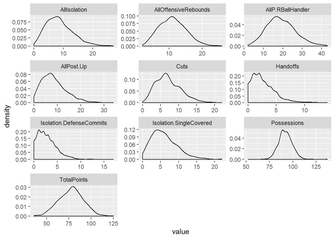
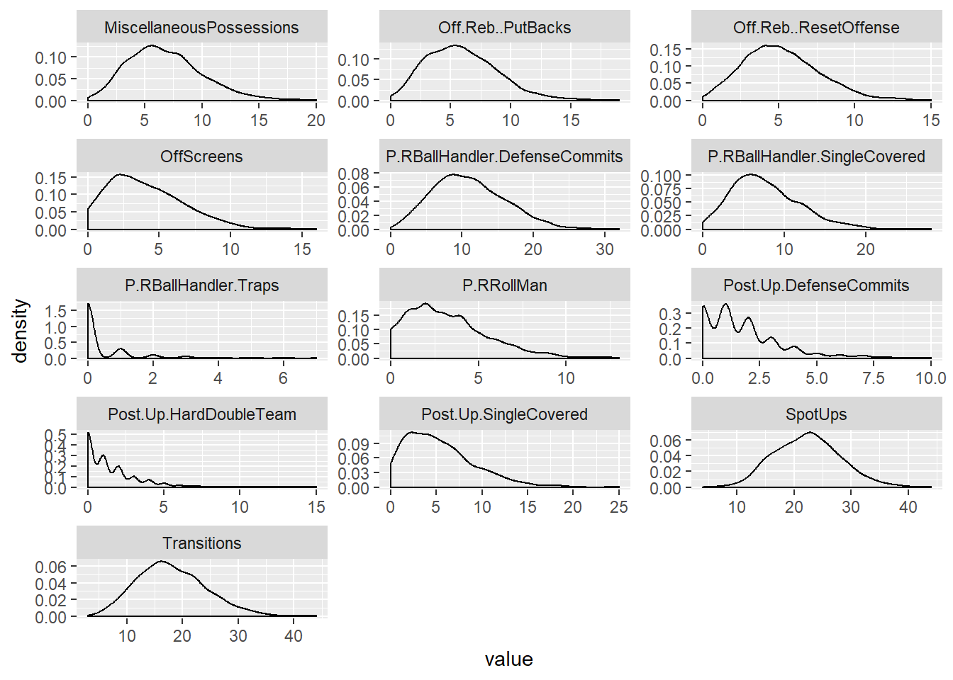
Figure 2.1: Distribution of PlayTypes Features.
The distributions of most of the Isolation, Post-Up and Pick and Roll plays are skewed to the right, along with Handoffs, Offscreens and Miscellaneous Posssessions. The rest of the plays are approximately normal.
Note: There is a difference in number of games per season because the number of games played per season increased from 19-20 games to 23-24 games in 2017/2018.
2.1.2 Outliers
An outlier is defined as a sample or event that is very inconsistent with the rest of the data set. However, in sports outliers are not due to measurement errors, they are due to teams playing differently against other teams.
2.1.3 Win/Loss Associations
2.1.4 Covariation
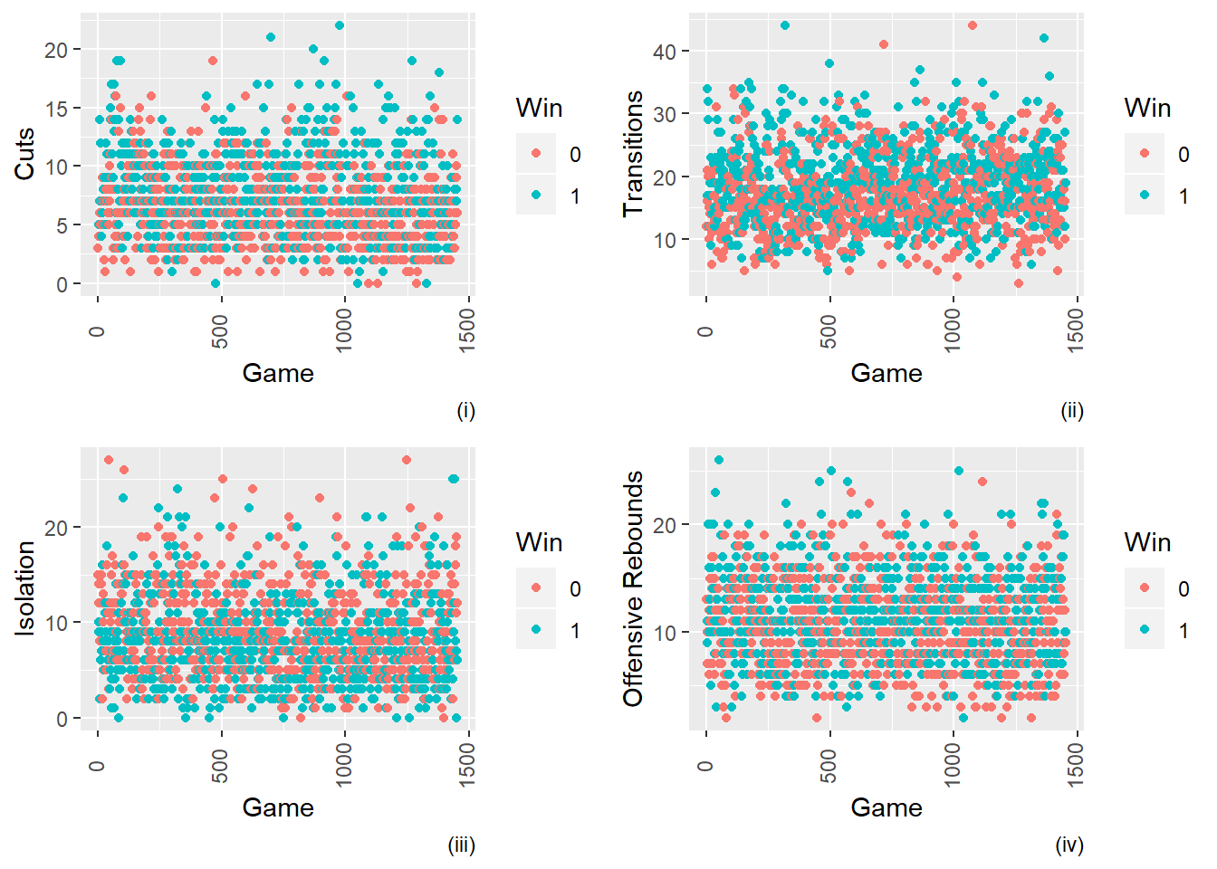
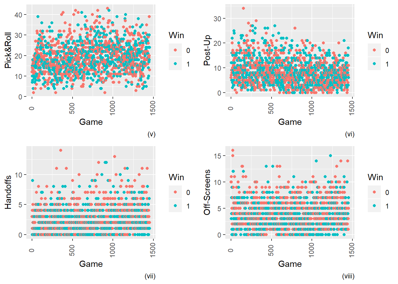
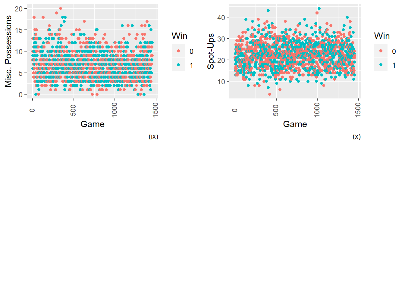
Figure 2.2: Scatterplots of certain Play Types vs. Wins (1) or Losses (0)
There is no clear pattern of any individual play type in respect to wins. This makes sense since different teams have different styles of play and have to adjust to their opponents’ style of play. It would make more sense to see the differentials for each game. For instance, if a team is not as tall as another team, the taller team may want to post-up more since they would have the advantage. This advantage may make the team more likely to win.
2.1.5 Sets
Below are the basic summary statistics of the Sets dataset which shows the number of times a team sets up their offense and where and when they do. Again, the reader can refer to Table 1.2 for the features and their associated descriptions. It may seem like there is an anomaly with the half-court vs zone variables but this is due to zone defense not being a popular defensive style in the league so when a team plays zone defense for the entire game then the opposing team will have to set their offense against it. We can see that zone defenses have right skewed distributions which further shows that zone defense is not a popular defensive style in U Sports Basketball.
| mean | sd | median | min | max | range | |
|---|---|---|---|---|---|---|
| AfterTimeOuts.ATO. | 8.637741 | 2.0509452 | 9.0 | 1 | 17 | 16 |
| HalfCourtSetAll | 74.034435 | 7.3461373 | 74.0 | 40 | 113 | 73 |
| HalfCourtSetAll.NoPts | 46.580579 | 7.0841925 | 46.0 | 24 | 73 | 49 |
| HalfCourtSetAll.Pts | 27.453857 | 5.2931895 | 27.0 | 11 | 48 | 37 |
| HalfCourtSetvs.Zone.NoPts | 2.807851 | 5.7575283 | 1.0 | 0 | 46 | 46 |
| HalfCourtSetvs.Man | 69.700413 | 10.8398110 | 71.0 | 6 | 113 | 107 |
| HalfCourtSetvs.Man.NoPts | 43.772727 | 8.7634901 | 44.0 | 4 | 71 | 67 |
| HalfCourtSetvs.Man.Pts | 25.927686 | 5.7791545 | 26.0 | 1 | 45 | 44 |
| HalfCourtSetvs.Zone | 4.334022 | 8.5731538 | 1.0 | 0 | 77 | 77 |
| HalfCourtSetvs.Zone.Pts | 1.526171 | 3.0937572 | 0.0 | 0 | 32 | 32 |
| Last4Sec.ofShotClock | 7.323003 | 3.4618639 | 7.0 | 0 | 20 | 20 |
| OutofBounds | 9.828512 | 3.1749254 | 10.0 | 1 | 23 | 22 |
| OutofBounds.End. | 5.244490 | 2.4351274 | 5.0 | 0 | 15 | 15 |
| OutofBounds.Side. | 4.584022 | 2.2218062 | 4.0 | 0 | 12 | 12 |
| TotalPoints | 77.440083 | 13.5884622 | 78.0 | 36 | 125 | 89 |
| Win | 0.500000 | 0.5001723 | 0.5 | 0 | 1 | 1 |
| Season* | 2.603306 | 1.1111564 | 3.0 | 1 | 4 | 3 |
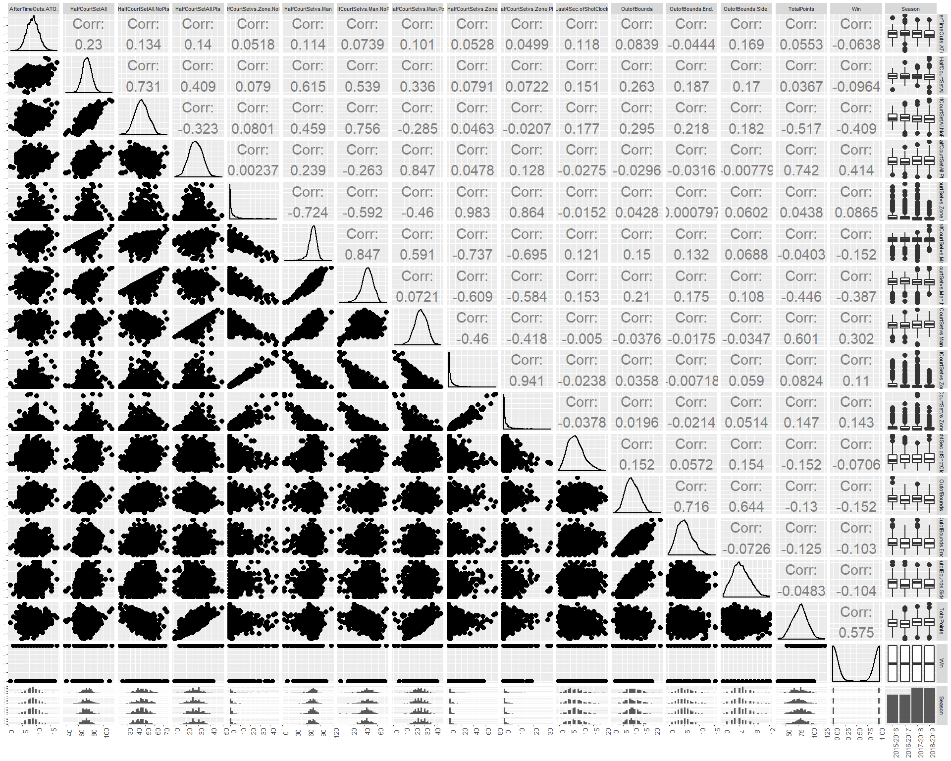
Figure 2.3: Plot Matrix of Sets Dataset.
2.1.6 Shots
Below are summary statistics of the Shots dataset (features and associated description are given in Table 1.3). From this we can see that on average, teams take more guarded shots than unguarded shots. Teams also take more long jump shots on average compared to short or medium jump shots. The average FG% from all teams from all 1488 games in the dataset is 27.75/68.1 = 40.75%. Teams on average attempt 25 3-Pointers and make about 8 per game which gives an average 3FG% of 32%; 2-Pointers have a higher efficiency on average because they are easier to score. Total Points are negatively correlated to guarded jump shots, short jump shots and medium jump shots, and are positively correlated to long jump shots (3 Pointers). It is self-explanatory that total points are negatively correlated to guarded shots as these have a higher likelihood of being missed. On the other hand, it is interesting to note that teams with players that take more short and medium jump shots as opposed to long shots have less total points, while teams with players taking more long jump shots have more total points. This shows that players with good 3-point shooting efficiency are highly valuable to a team and may in fact be an important factor to a team’s season performance.
| mean | sd | median | min | max | range | |
|---|---|---|---|---|---|---|
| X2FG.Attempts | 43.172865 | 7.9905014 | 43.0 | 19 | 76 | 57 |
| X2FG.Made | 19.894628 | 5.2749932 | 20.0 | 5 | 37 | 32 |
| X2FG.Missed | 23.278237 | 6.1437855 | 23.0 | 6 | 46 | 40 |
| X3FG.Attempts | 25.135675 | 6.5643332 | 25.0 | 8 | 47 | 39 |
| X3FG.Made | 7.883609 | 3.2277794 | 8.0 | 0 | 23 | 23 |
| X3FG.Missed | 17.252066 | 5.0190364 | 17.0 | 4 | 40 | 36 |
| All.Free.Throws | 19.064738 | 7.0358888 | 18.0 | 0 | 44 | 44 |
| FG.Attempts | 68.308540 | 7.8644519 | 68.0 | 40 | 102 | 62 |
| FG.Made | 27.778237 | 5.7206141 | 28.0 | 12 | 51 | 39 |
| FG.Missed | 40.530303 | 7.0999397 | 40.0 | 16 | 68 | 52 |
| Guarded.Jump.Shots | 12.511708 | 5.5112691 | 12.0 | 1 | 31 | 30 |
| Live.Free.Throws | 10.068870 | 3.6851550 | 10.0 | 0 | 23 | 23 |
| Long.Jump.Shots..3.point.shots. | 25.351240 | 6.5999639 | 25.0 | 8 | 48 | 40 |
| Medium.Jump.Shots..17..to..3.point.line. | 4.294766 | 2.8733717 | 4.0 | 0 | 19 | 19 |
| Short.Jump.Shots…17.. | 4.687328 | 2.9039348 | 4.0 | 0 | 16 | 16 |
| Total.Points | 77.440083 | 13.5884622 | 78.0 | 36 | 125 | 89 |
| Unguarded.Jump.Shots | 8.913223 | 4.8063152 | 8.0 | 0 | 27 | 27 |
| Win | 0.500000 | 0.5001723 | 0.5 | 0 | 1 | 1 |
| Season* | 2.603306 | 1.1111564 | 3.0 | 1 | 4 | 3 |
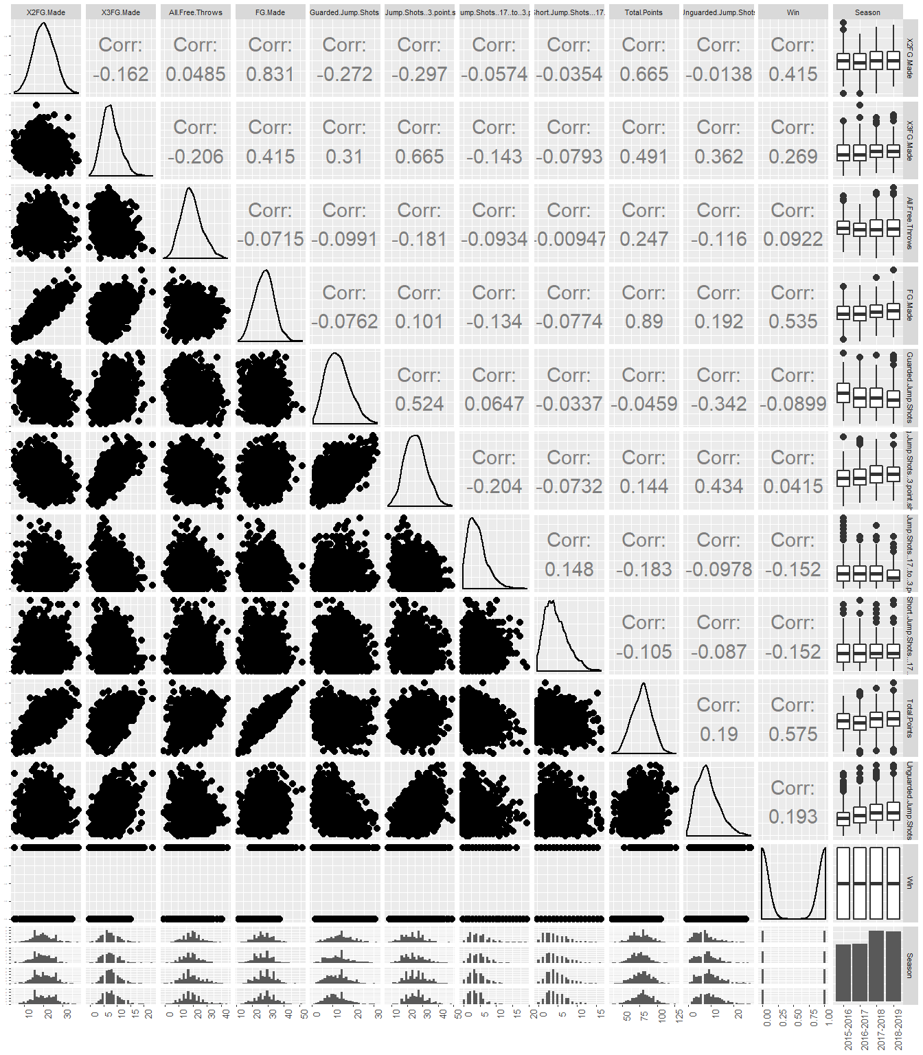
Figure 2.4: Plot Matrix for Shots Dataset
2.1.7 Visualizations
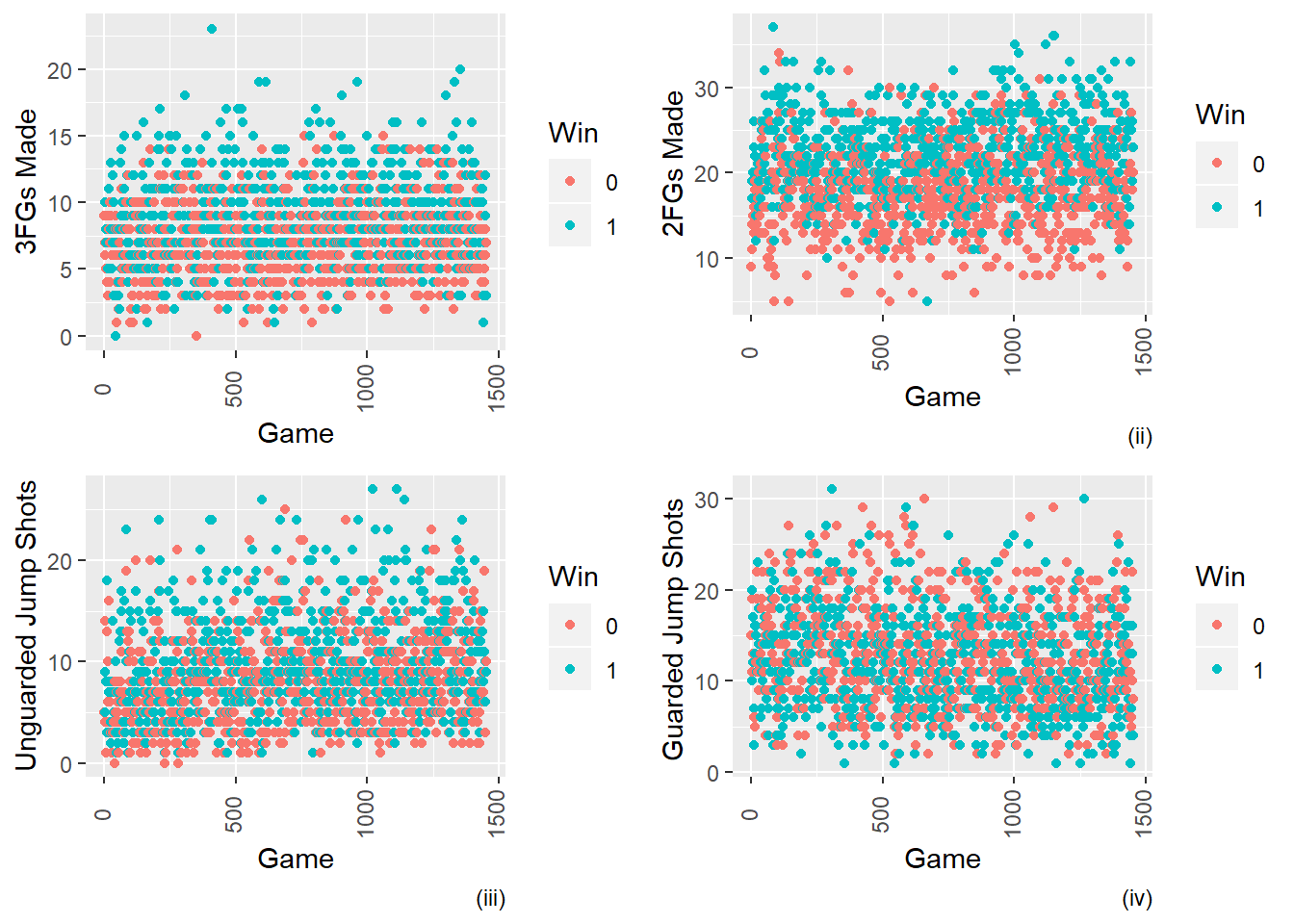
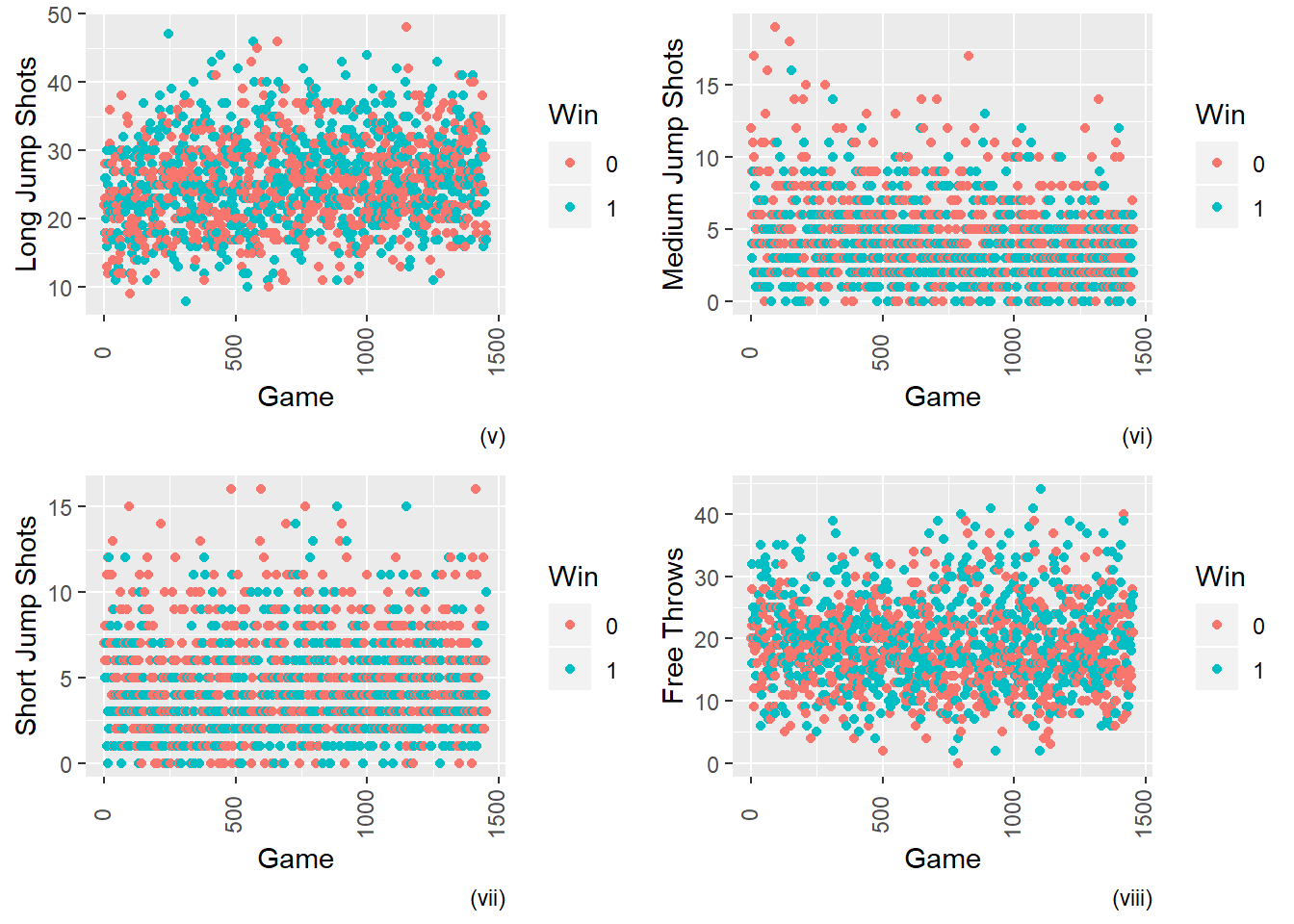
Figure 2.5: Comparing Shot Types vs. Wins(1) or Losses(0)
From the above figure, we can see that more unguarded shots (iii) is more highly associated to wins compared to guarded shots (iv). In this figure we can see that taking a lower number of medium jump shots (vi) contribute to more wins as opposed to the other types of shots (v & vii) that are taken.
2.1.8 Transitions
Below are summary statistics of the Transitions dataset (features and associated descriptions are given in Table 1.4). Total Points is most positively correlated to Transition Offense with 0.36 where Transition Offense occurs when a team gains possession of the ball and quickly pushes it to the opposing team’s basket. Total Points is most negatively correlated to Press Offense. Press Offense is when the offense (the team having possession of the ball) is being pressed by the other team, i.e. they are being defensively pressured in which members of the defense cover their opponents throughout the court and not just near their own basket. Being pressured would make it harder to score, thus why it is the most negatively correlated to points. The outliers (shown in the boxplots) are all on the upper tails and may be due to the pace of game having a big variance. For example, a team may have a higher Transition Offense rate when the pace of the game is fast, but if the pace is slow, they may not transition from defense to offense as often. The outliers should not be removed from the dataset since they are not measurement errors and provide useful information where the data points largely deviate from the average.
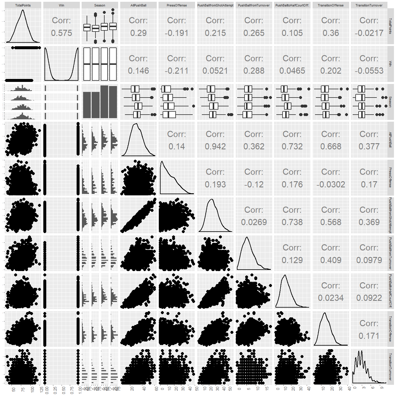
Figure 2.6: Plot Matrix of the Transitions Dataset
2.1.9 General Statistics
2.1.10 Home Vs. Away
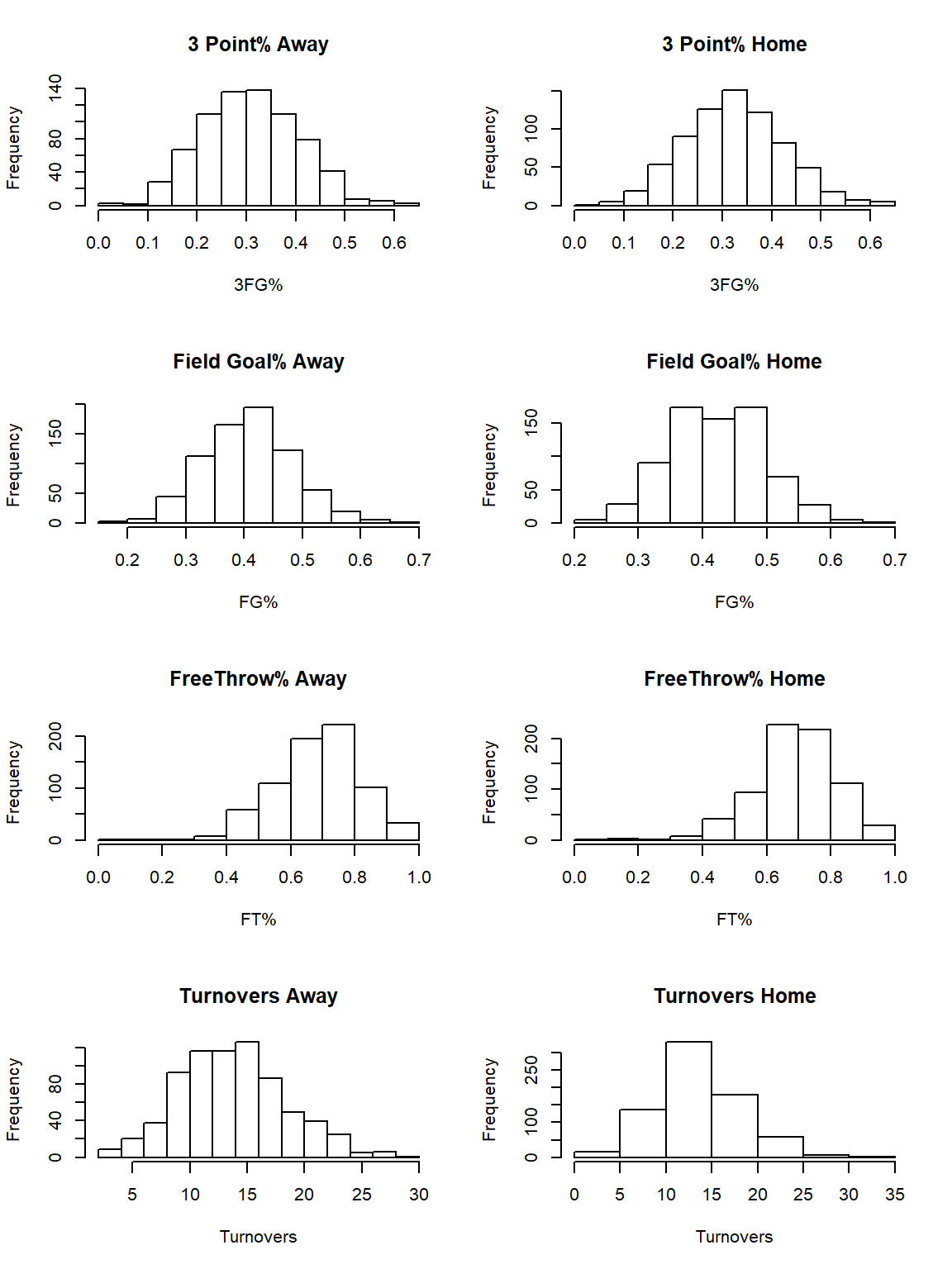
Figure 2.7: Distribution of Variables; Away vs. Home
The distributions for the home variables vs the away ones are very similar, however there is a slight difference between the Field Goal Percentage.
| Average | Statistic | |
|---|---|---|
| Away | 0.4092 | FG% |
| Home | 0.4228 | FG% |
| Away | 0.3123 | 3FG% |
| Home | 0.3281 | 3FG% |
There is a very slight difference between the home and away field goal percentages but does this mean that there is a home court advantage?
| Home Wins | Away Wins |
|---|---|
| 402 | 328 |
This shows there is a difference between the number of times a home team wins compared to an away team.
2.1.11 Risk Ratios and Odd Ratios
2.1.11.1 What are Risk Ratios and Odd Ratios
Risk Ratio (RR) or Relative Risk is a measurement often used in epidemiology. It is used to estimate the outcome between factors and outcomes. In our case we will use this measurement to see whether there is a statistically significant difference between teams playing at home versus away. A risk ratio of 1 means there is no difference, greater than 1 means there is a higher chance of winning if the team is playing at home, and less than 1 means the opposite [4]. An Odds Ratio (OR) is a ratio of ratios. It also quantifies the strength of the association between two events. If the odds ratio equals 1 then the odds of the events are the same. If the odds ratio is greater than 1 then the events are correlated in the sense that if compared to the absence of the second event, the presence of the second raises the odds of the first event, and symmetrically the presence of the first event raises the odds of the second event. In our case we will obtain both measurements to see the strength of association between teams playing at home versus teams playing away.
2 by 2 table analysis:
------------------------------------------------------
Outcome   : Win
Comparing : Home vs. Away

     Win Lose    P(Win) 95% conf. interval
Home 402  328    0.5507    0.5144   0.5864
Away 328  402    0.4493    0.4136   0.4856

                                   95% conf. interval
             Relative Risk: 1.2256    1.1049   1.3595
         Sample Odds Ratio: 1.5021    1.2222   1.8462
Conditional MLE Odds Ratio: 1.5017    1.2156   1.8562
    Probability difference: 0.1014    0.0501   0.1519

             Exact P-value: 0.0001
        Asymptotic P-value: 0.0001
------------------------------------------------------
The probability of winning at home is 55% whereas the probability of winning away is 45%. The Sample Odds Ratio tells us that odds of a team winning is 1.5 higher given they are playing at home compared to playing away. The Relative Risk tells us that home teams have 1.22 times the ‘risk’ of winning compared to away teams.
A coach may be more interested in which teams in particular play better at home, and how much better they play.
2.1.11.2 Home vs. Away by Team

Figure 2.8: Difference of Home Statistics vs. Away Statistics of the 2018-2019 Season for each team.
Above is a table of the every team from the 2018-2019 season where the Home statistics are all subtracted by the Away Statistics, i.e. the statistics of a team when they were playing at home subtracted by statistics when they were playing away. A positive number indicates that the team performed better at home (except for turnovers). For example, Carleton shot their free throws 8.91% higher at home.
2.1.11.2.1 Insights
The top 3 teams that shot their free thows better at home are Western (12.32%), Carleton (8.91%), and Lakehead (5.58%). The top 3 teams that shot field goals better at home are Ottawa (6.44%), Toronto (5.59%), and Windsor (4.88%). The top 3 teams that shot 3 pointers better at home are Ottawa (11.20%), Laurentian (8.18%), Nipissing (5.69%). The top 3 teams that turnover the ball the least when playing at home are Algoma (-3.17), Western (-2.75), and Laurentian (-2.65). The top 3 teams that rebound the ball more at home are Ryerson (10.64), Brock (9.08), and Laurentian (6.11). The top 3 teams that scored more points at home are Ottawa (12.11), Toronto (10.89), and Laurentian (9.74). On average, the teams turned over the ball 6 less times at home,
2.1.11.2.2 Conclusion
In conclusion, many teams benefit from playing at home, and different teams excel differently. According to a Bleacher Report study [5], referee bias and the psychological impact of playing at home are two of the biggest factors of why there is a large difference between home and away statistics. Studies have show that when a crowd is vocal, it impacts the way referees call a game. Also, referees have historically favored home teams. In addition, the psychological impact of playing at home is a self-sustaining placebo effect: Home-court advantage gives the home team an edge simply because players believe that it does.
2.1.12 Wins Per Season
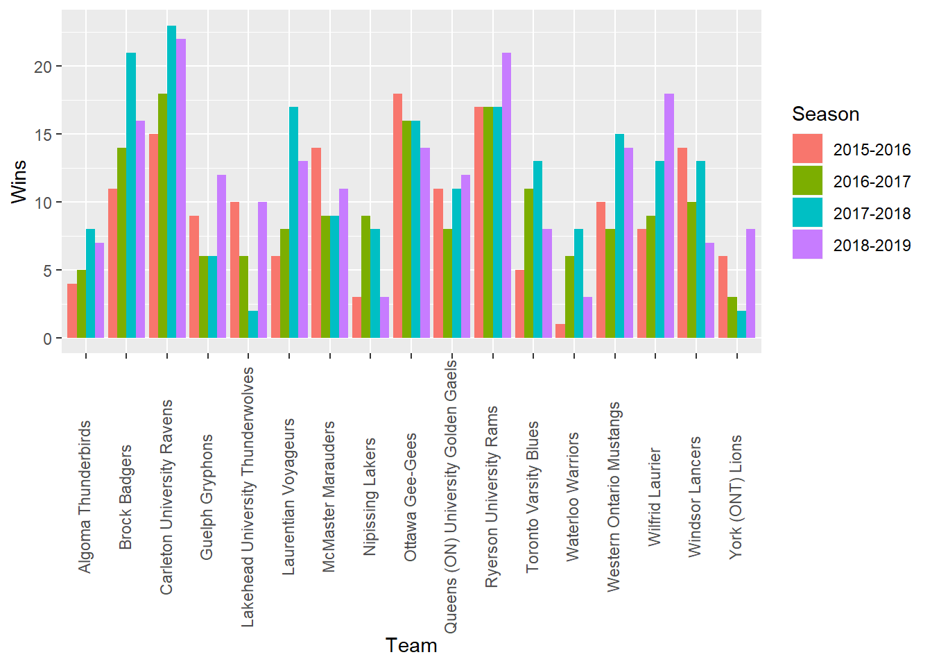
Figure 2.9: Wins per Season for all teams in the OUA division
The above shows that Brock, Carleton, Laurentian, UofT, and Western all steadily improved and peaked at the 2017-2018 season. The Ryerson Rams stayed consistent and peaked 2018-2019 season. There are few teams that are consistently not winning more than 10 games a season such as Algoma, Nipissing and York.
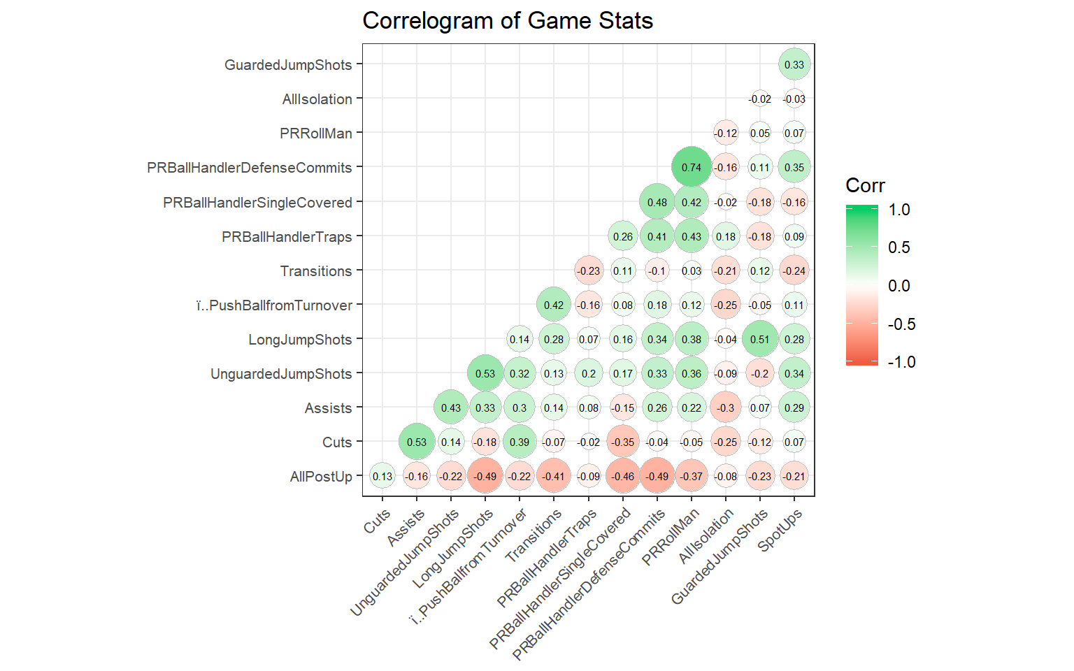
2.2 Correlations
The table below gives the correlations between different Play Types and Total Points scored in a game. Note that a negative number represents a negative correlation between the two features while a positive number represents a positive correlation. A correlation measurement closer to 0 represents a non-linear relationship as opposed to a correlation measurement further from 0.
| Play Type | Correlation to Total Points |
|---|---|
| All Isolation | -0.046532124 |
| All Offensive Rebounds | 0.154450763 |
| All PR Ball Handler | 0.042544034 |
| All Post-Up | -0.040890549 |
| Cuts | 0.227413916 |
| Handoffs | -0.017105738 |
| Isolation Defense Commits | -0.045338194 |
| Isolation Single Covered | -0.032922237 |
| Miscellaneous Possessions | -0.075670507 |
| OffScreens | -0.135119217 |
| Offensive Rebound Putback | 0.154161317 |
| Offensive Rebound Reset Offense | 0.067340925 |
| PR Ball Handler Defense Commits | 0.053122283 |
| PR Ball Handler Single Covered | 0.013881865 |
| PR Ball Handler Traps | -0.020176743 |
| PR Roll Man | 0.101940646 |
| Post Up Defense Commits | -0.056702755 |
| Post Up Hard Double Team | -0.090199983 |
| Post Up Single Covered | 0.013534056 |
| Spot Ups | -0.007428537 |
| Transitions | 0.317687812 |
The plays that are most positively correlated to total points are transitions, cuts, and offensive rebounds. This could mean that transitions, cuts and offensive rebounds contribute to the most points compared to all other plays. The play that is most negatively correlated to total points is offscreens.
To account for outliers and since some teams have played more a game or two more than others, the dataset was transformed by averaging the statistics per game per season, and the wins were summed.
| Features | Correlation to Number of Wins |
|---|---|
| Press Offense | -0.175526612 |
| Push Ball From Shot Attempt | 0.091290517 |
| Push Ball From Turnover | 0.484877383 |
| Push Ball to Half Court | 0.115357730 |
| Free Throws | -0.092037012 |
| Guarded Jump Shots | -0.153775302 |
| Unguarded Jump Shots | 0.592888473 |
| Long Jump Shots | 0.331422037 |
| Medium Jump Shots | -0.365731181 |
| Short Jump Shots | -0.197920494 |
| Cuts | 0.373973357 |
| Handoffs | -0.072249207 |
| Isolation Single Covered | -0.354371026 |
| Isolation Defense Commits | -0.006820286 |
| Miscellaneous Possessions | -0.406512329 |
| OffScreens | -0.280720057 |
| Offensive Rebound PutBack | 0.166641468 |
| Offensive Rebound Reset | 0.368757978 |
| PR Ball Handler Defense Commit | 0.338107184 |
| PR Ball Handler Single Covered | 0.072595284 |
| PR Ball Handler Traps | 0.115888712 |
| PR Roll Man | 0.311420152 |
| Post Up Defense Commits | -0.171605486 |
| Post Up Hard Double Team | -0.067993980 |
| Post Up Single Covered | -0.183923948 |
| Spot Ups | 0.247910273 |
| Transitions | 0.231836305 |
| Assists | 0.653151380 |
| Blocks | 0.337827582 |
| Steals | 0.490803284 |
| Total Rebounds | 0.447741075 |
| Turnovers | -0.319146688 |
