Chapter 7 Week 9 - Factorial ANOVA
Outline:
- Analysis Of Variance Continued
Treatment Designs: Factorial ANOVA
- The Treatment Design Concept
- The Factorial Alternative - How to Waste resources??
- What is this ‘Interaction’??
- The Factorial Model
- Factorial Effects
- The Factorial ANOVA
- Partitioning Treatment Sums of Squares Into Factorial Components
- Factorial Effects and Hypotheses
- Testing and Interpreting Factorial Effects
- Using R
- Using R for Factorial ANOVA
Accompanying Workshop - done in week 10
- Defining factorial treatments.
- The analysis of variance for factorial treatment designs – by hand and using R
Workshop for week 9
- Based on lectures in week 8
- Response to marker’s critique. Designed to help you improve in your assignment 2.
Project Requirements for Week 9
- Assignment 2 is available on Learning@Griffith from this week (week 9). It is due in week 11.
7.1 Treatment Designs: Factorial ANOVA
7.1.1 The Treatment Design Concept
The treatments involved in a study often involve several factors. Interest will then lie in the effects of each of the factors and in the possible interaction between the factors.
Example: Environmental Monitoring
An environmental monitoring system treatment may consist of two components: the machine used and the degree of instructions given to the operator. Suppose these are:
- 4 degrees of instruction - 0, small (S), standard (M) and extra (E)
- 3 types of machine - A, B and C
The treatments will be made up of all combinations of the two factors.
Treatment Degree of Instruction Type of Machine 1 0 Instruction Machine A 2 3 4 5 6 7 8 9 10 11 12
The different possible values for a factor are known as its levels. In the example, degree of instruction has 4 levels and type of machine has 3 levels. The total number of treatments will be the product of the levels of the factors involved: \(4 \times 3 = 12\).
Standard Order - ABC
When trying to identify all treatments from a number of factors, it is useful to have some standard approach – this avoids missing treatments along the way!! A commonly used approach is known as the ‘standard ABC order’ in which the levels of the first factors (A and B) are held constant while the levels of the outermost factor (C) are allowed to vary. Once all levels of C have been varied for a particular combination of A and B, the level of the next factor, B, is varied and C again moves through its possible levels. Eventually factor B will reach its last level together with the last level of C, only then will the level of A change. The process with factors B and C then repeats but with the second level of A.
Assuming there are ‘a’ levels of A, ‘b’ levels of B and ‘c’ levels of C, the \(a \times b \times c\) treatments can be written schematically as: A1B1C1, A1B1C2, …, A1B1Cc, A1B2C1, A1B2C2, …, A1B2Cc, …, A1BbCc, A2B1C1, A2B1C2, …, A2B2Cc, A2B2C1, A2B2C2, …, A2BbCc, …, AaBbCc.
Example: Air Pollution, Land Usage, and Location
Three land uses (rural, residential and national park)
Two states (Qld and NSW)
7.1.2 The Factorial Alternative - How to Waste resources?
The alternative to the factorial design in the environmental monitoring example above would involve several experiments.
instruction level 0: 3 machine types, each replicated a minimum of 5 \(\rightarrow\) 15 units
instruction level S: 3 machine types, each replicated a minimum of 5 \(\rightarrow\) 15 units
instruction level M: 3 machine types, each replicated a minimum of 5 \(\rightarrow\) 15 units
instruction level H: 3 machine types, each replicated a minimum of 5 \(\rightarrow\) 15 units
machine type A: 4 instruction levels, each replicated a minimum of 4 \(\rightarrow\) 16 units
machine type B: 4 instruction levels, each replicated a minimum of 4 \(\rightarrow\) 16 units
machine type C: 4 instruction levels, each replicated a minimum of 4 \(\rightarrow\) 16 units
A total of seven separate experiments, using a total of (\(4 \ times 15\)) + (\(3 \times 16\)) = 108 experimental units.
AND still no quantitative measure of the interactive effect of the degree of instruction and the machine type.
When all possible combinations are used the design is called a complete factorial.
Incomplete factorials are a valuable design; can save resources – but not covered here.
7.1.3 What is this ‘Interaction’??
The best way to understand the ‘interaction’ concept is to look at an example.
Example: Chemicals and Weed Control
A controlled laboratory experiment has been carried out to look at the effects of four different chemicals on the control of a noxious weed. Since it was unknown whether the chemical effect would depend on the stage of development of the plant at the time of application, some plants were treated in an early stage of growth and others later in their growing process.
Each chemical was applied to six experimental plants, three in early growth stage and three in late growth, giving a total of 24 experimental plants. Each chemical was applied at the concentration recommended by the manufacturers. For confidentiality purposes, the chemicals are known simply as A, B, C and D.
The variable measured was dry matter production at six weeks of age. The results for the 24 individuals are given below.
Time of Application A B C D Time of Application Total 5.9 2.6 4.7 2.0 Early 4.7 3.7 4.3 2.4 5.6 (16.2) 3.4 (9.7) 3.8 (12.8) 1.9 (6.3) 45.0 2.5 2.7 3.1 5.9 Late 0.6 2.3 4.1 4.6 1.0 (4.1) 2.9 (7.9) 2.8 (10) 5.5 (16.0) 38.0 Chemical Total 20.3 17.6 22.8 22.3 83.0 There are 8 different sets of three individuals – representing 8 different treatments. The two way table of means identifies the mean values for these 8 sets:
Time of Application A B C D Time Means Early 5.4 3.2 4.3 2.1 3.8 Late 1.4 2.6 3.3 5.3 3.2 Chemical Means 3.4 2.9 3.8 3.7 Grand Mean 3.5 Looking at the means for the different chemicals for the two times and overall gives:
drymatter<- c(5.9, 4.7, 5.6, 2.5, 0.6, 1,
2.6, 3.7, 3.4, 2.7, 2.3, 2.9,
4.7, 4.3, 3.8, 3.1, 4.1, 2.8,
2, 2.4, 1.9, 5.9, 4.6, 5.5)

time <- factor(rep(rep(c("Early", "Late"), c(3, 3)), 4))
chemical <- factor(rep(LETTERS[1:4], rep(6, 4)))

# Put variables in a dataframe and clean up:
weeds <- data.frame(drymatter, time, chemical)
rm(drymatter, time, chemical)

attach(weeds)
interaction.plot(chemical, time, drymatter, type = "l", col = c("blue", "red"), main = "Interaction Plot for Weed Control Example")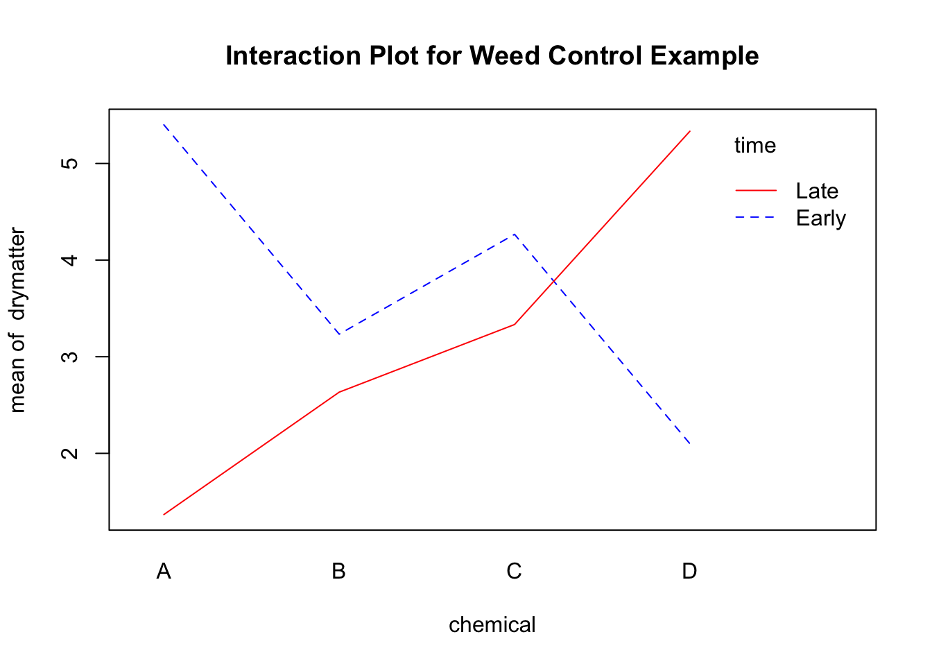
The differences between the chemicals clearly depend on whether the application occurred during the early or late stage of growth. If application is in the early growth stage, chemical D appears to be more effective as it produces much less dry matter of weed; but if application is in the later growth stage it is chemical A which is more effective, and chemical D is the worst of the chemicals (weeds treated with D have a high average production). The effect of chemicals interacts with the time of application – the effect of the chemicals depends on which time of application is being considered.
What about the question of whether it is better to apply the chemical in the early stages of growth or hold off until a later stage?
7.1.4 The Factorial Model
Factorial Model
When more than one factor is involved the model used to describe the dependent variable will involve terms for each factor and also terms for possible interactions between the various factors. The following general model would apply for two factors, say A and B, with \(a\) and \(b\) levels, respectively:
\[ y_{ijk} = \mu + \alpha_i + \beta_j + \alpha\beta_{ij} + \epsilon_{ijk}, \]
where
- \(y_{ijk}\) is the observation on the \(k\)th replicate receiving the \(i\)th level of A and the \(j\)th level of B, \(k = 1, \ldots, n\);
- \(n\) is the number of replicates for each of the \(a \times b\) treatment groups;
- \(\mu\) is the overall grand mean of y;
- \(\alpha_i\) is the effect of the \(i\)th level of factor A, \(i=1, \ldots, a\);
- \(\beta_j\) is the effect of the \(j\)th level of factor B, \(j=1, \ldots, b\);
- \(\alpha\beta_{ij}\) is the effect of the interaction between factor A and B;
- \(\epsilon_{ijk}\) is the random effect attributable to the ijkth individual observation.
Notes
- The index, \(k\), counts the replicates for a particular treatment group and goes from 1 to n. (There are \(a \times b\) treatment groups, each replicated n times).
- Each level of factor A is replicated not only by each group of n, but also across the levels of factor B – overall each level of A has \(b \times n\) replicates. Similarly, levels of factor B gain replication because they occur at the different levels of factor A – overall each level of B has \(a \times n\) replicates. It is the replication of one factor’s levels across the levels of the other factor that gives the factorial treatment design its power. As long as everything is balanced, and all levels of one factor are represented equally in all levels of every other factor, then any effect due to one factor is ‘evened’ out when another factor’s levels are being compared.
Preliminary Model
It is useful to consider an initial model which contains a single treatment term encompassing all the factorial effects (both main and interaction). Such a model is known as a preliminary model. One of the advantages of this model is to ascertain the sources of variation which will be unexplained (error) and the sources that will form part of the experimental design (for example, blocking). This will be discussed further in courses in later years.
The preliminary model for the general two-factor model above is:
\[ y_{ijk} = \mu + \text{treat}_{ij} + \epsilon_{ijk} \]
where
- \(y_{ijk}\), \(\mu\), and \(\epsilon_{ijk}\) are as previously defined;
- \(\text{treat}_{ij}\) is the effect of the \(ij\)th treatment group (made up from the factors A and B), \(i= 1, \ldots, a\) and \(j=1, \ldots, b\).
7.1.5 Factorial Effects
When the treatment effect in the preliminary model is partitioned to provide the factorial components of the treatment, two types of terms appear – main effect terms and interaction terms.
A main effect represents the effect of the identified factor on average across all levels of any other factors.
An interaction effect is a measure of any additional contribution arising from the interaction of one factor with another (or others). If two factors act independently of each other their interaction will be zero; the contribution made by any one of them in the make-up of the observation is through the values of its individual levels, regardless of the level of the other factor.
7.1.6 The Factorial ANOVA
The PROJECTED ANOVA
A projected ANOVA is a very useful design tool. It consists of the source of variation together with the degrees of freedom associated with each source. Data from an experiment, which has been designed using a projected ANOVA, will fall automatically into an appropriate analysis. In the factorial ANOVA sources of variation will come from main effects and interaction effects, and degrees of freedom will be needed for each type of effect.
For main effects the degrees of freedom are those that would apply if the factor were a treatment – that is, the degrees of freedom will be one less than the number of levels.
For interaction effects the degrees of freedom are the product of the degrees of freedom of the factors in the interaction.
Preliminary Projected ANOVA (Balanced):
| Source of Variation | Degrees of Freedom |
|---|---|
| Treatments | \(ab - 1\) |
| Error | \(ab(n - 1)\) |
| Total | \(abn - 1\) |
Factorial Projected ANOVA (Balanced):
| Source of Variation | Degrees of Freedom |
|---|---|
| Main Effect A | \(a - 1\) |
| Main Effect B | \(b - 1\) |
| Interaction A and B | \((a - 1) \times (b - 1)\) |
| Error | \(ab(n - 1)\) |
| Total | \(abn - 1\) |
Example: Chemicals and Weed Control (Contd.)
Recall the previous example where the effects of three different chemicals on the control of a noxious weed were studied. Each chemical will be applied at a standard concentration at two different times of growth, early and late. Forming a complete factorial will require 8 treatments: 4 chemicals \(\times\) 2 times. There were 3 replicates within each treatment. The variable measured is dry matter production (production).
Preliminary Model:
\[ \text{production}_{ijk} = \mu + \text{treat}_{ij} + \epsilon_{ijk} \]
Factorial Model:
\[ \text{production}_{ijk} = \mu + \text{Ch}_i + \text{apptime}_j + (\text{Ch} \times \text{apptime})_{ij} + \epsilon_{ijk}, \]
where - \(\text{production}_{ijk}\) is the observed dry matter production on the \(k\)th replicate of the \(i\)th chemical applied at the \(j\)th application time; - \(\text{Ch}_i\) is the effect of the \(i\)th chemical, \(i=1, \ldots, 4\); - \(\text{apptime}_j\) is the effect of the \(j\)th application time, \(j=1, 2\); - \((\text{Ch} \times \text{apptime})_{ij}\) is the effect of the interaction between chemical and application time; - \(\epsilon_{ijk}\) is the unexplained component of the \(ijk\)th observation. \(k = 1, 2, 3\).
In words, the model says, the amount of dry matter production in the ijkth replicate (observation) is due to the \(i\)th chemical, the \(j\)th time of application, the possible two way interaction between these two factors and any inherent variation associated with that particular replicate (observation).
Projected ANOVAs (to be completed in lectures)
Preliminary:
Source of Variation Degrees of Freedom Treatments Error Total Factorial:
Source of Variation Degrees of Freedom Chemical Applicaction Time Ch \(\times\) AppTime Error Total
7.1.7 Partitioning Treatment Sums of Squares Into Factorial Components
The sums of squares for the factorial ANOVA are found using a two stage approach which parallels the projected ANOVA process. For a case of two factors the process is as follows.
- Stage 1:
- The SS for the treatments are found as usual – this value is the preliminary treatment sums of squares which must then be partitioned into its component parts as determined by the factorial design.
- Stage 2 A:
- For each main effect, the sums of squares is found by regarding the factor as a treatment – the total for each level of the factor is squared and divided by the number of observations in that level (note that any other factors are completely ignored at this stage); these modified totals are then added and the Correction Factor is subtracted, as for the calculation of any treatment sums of squares.
- Stage 2 B:
- The interaction sum of squares is found by subtracting the main effect sums of squares from the preliminary treatment sum of squares.
Example: Chemicals and Weed Control (contd):
Return to the example on the chemicals and weed control. The Total Sum of Squares, Treatment Sum of Squares and Residual Sum of Squares are calculated in the usual way as:
\[\begin{align*} \text{Total SS} &= \sum_i\sum_j y_{ij}^2 - \frac{(\sum_i\sum_j y_{ij})^2}{n} \\ &= \end{align*}\]
\[\begin{align*} \text{TSS = Treatment SS} &= \sum_i \frac{T_i^2}{n_i} - \text{CF} \\ &= \end{align*}\]
\[ \text{ESS = Residual Sum of Squares = Tot SS - TSS} = \]
\[\begin{align*} \text{Chemical SS} &= \frac{\text{(Total A)}^2}{3 + 3} +\frac{\text{(Total B)}^2}{3 + 3} + \frac{\text{(Total C)}^2}{3 + 3} + \frac{\text{(Total D)}^2}{3 + 3} - \frac{(\text{Total A + Total B + Total C + Total D})^2}{4 \times (3 + 3)}\\ &= \frac{20.3^2}{6} +\frac{17.6^2}{6} + \frac{22.8^2}{6} + \frac{22.3^2}{6} - \frac{(20.3 + 17.6 + 22.8 + 22.3)^2}{24}\\ &= 2.7883. \\ & \\ \text{Time SS} &= \frac{\text{(Total Early)}^2}{3 + 3 + 3 + 3} +\frac{\text{(Total Late)}^2}{3 + 3 + 3 + 3} + - \frac{(\text{Total Early + Total Late})^2}{2 \times (3 + 3 + 3 + 3)}\\ &= \frac{45.0^2}{12} +\frac{38.0^2}{12} - \frac{(45.0 + 38.0)^2}{24}\\ &= 2.0417. \\ & \\ \text{Interaction SS} &= \text{Treatment SS} - \text{Chemical SS} - \text{Time SS} \\ &= 44.7183 – 2.7883 – 2.0417 \\ &= 39.8883 \end{align*}\]
The ANOVAs are:
Preliminary:
Source DF SS MS VR Treatments 7 44.7183 6.3883 17.09 Error 16 5.9800 0.3738 Total 23 50.6983 Factorial:
Source DF SS MS VR Chemical 3 2.7883 0.92944 2.49 Time 1 2.0417 2.04167 5.46 Chemical \(\times\) Time 3 39.8883 13.29611 35.57 Error 16 5.9800 0.37375 Total 23 50.6983
7.1.8 Factorial Effects and Hypotheses
Factorial Effects
Each line of the Factorial ANOVA resulting from the partitioned treatment source of variation, provides a test of some hypothesis. This means that a factorial ANOVA with 2 main effects will need a null and alternative hypothesis for EACH of the main effects and for the interaction, i.e. 3 null and 3 alternative hypotheses will be needed.
A main effect line provides a test of the equality of means for the particular factor, where the mean for each level is computed across all levels of the other factors. It describes the effect of the factor when it is averaged across all levels of the other factors. In the above example ‘chemicals’ and ‘time appln’ are the 2 main effects.
An interaction line tests whether or not the two (or more) factors interact with each other; are the differences between the levels of one factor the same regardless of which level of the other factor is considered OR do the differences change, depending on which level of the other factor is being considered?
Hypotheses for Chemicals and Weed Control example:
Chemical Main Effect
\(H_0:\) (main effect 1):
\(H_1:\) (main effect 1):
Time of Application Main Effect
\(H_0:\) (main effect 2):
\(H_1:\) (main effect 2):
Interaction Between Chemical and Time of Application
\(H_0:\) (interaction):
\(H_1:\) (interaction):
CRITICAL NOTE
If an interaction is significant then the main effects for the factors in the interaction should NOT be considered in isolation.
7.1.9 Testing and Interpreting Factorial Effects
All tests are carried out by considering the appropriate variance ratio and applying it to an F-test.
Step 1:
- Consider the interactions working from the highest order down.
Step 2 A:
- If an interaction is significant, the factor means within it must be interpreted using the two-way (or three-way, etc) table of means. Each factor must be considered separately for each level of the other factor(s) - the example will clarify this.
Step 2 B:
- If a main effect is not involved in a significant interaction, then it is interpreted in the same way that a treatment effect would be interpreted.
Example Chemicals and Weed Control (contd. and completed):
Return to the previous example and assume that the required assumptions of, independence, homogeneity of variances, additivity of model terms and normality of the variable, dry matter production,are all valid.
Interaction
\(H_0\): there is no interaction between chemicals and time of application – the effects of chemicals and time of application are independent.
\(H_1\): there is an interaction between chemicals and time of application – the effects of chemicals depend on the level of time of application, and vice versa.
Under \(H_0\), the \(VR \sim F_{3,16}\). From tables, \(F_{3,16}(0.95) = 3.24\). The critical region is \(VR \geq 3.24\).
Calculated VR of \(35.57\) lies in critical region therefore \(H_0\) is rejected and we conclude that there is a significant interaction between chemicals and time of application (\(p < 0.05\)). Further testing should be carried out on the two way table of means and not on the main effect means. This means we do not comment on the significance of the main effects in the ANOVA table or interpret them.
Interpretation of two way table of means (used to further test the significant interaction)
Find the least significant difference needed between any two of the 8 treatment means for the difference to be significant.
Standard deviation:
best estimate is square root of error mean square in the ANOVA: sd = 0.61135
Number of replicates in each treatment:
for the two-way (treatment) means there are 3 replicates
Standard error of difference between 2 means:
\[\begin{align*} SE_{\bar{y}_i - \bar{y}_j} &= s \times \sqrt{\frac{1}{n_i} + \frac{1}{n_j}} \\ &= 0.61135 \times \sqrt{\frac{2}{3}} \\ &= 0.499 \end{align*}\]
LSD(0.05) = \(t_{16}(0.975) \times \text{SEdiff means} = 2.12 \times 0.499 = 1.058\)
The means need to be 1.06 units apart before the treatment means are said to be significantly different at the 5% level of significance. Look at the graph of the means in section 1.3.
Considering the means for the chemicals (to be completed in lectures):
Early Application:
Late Application:
Considering the means for the time of application (to be completed in lectures):
Chemical A:
Chemical B:
Chemical C:
Chemical D:
Conclusions(to be completed in lectures):
7.2 Using R for Factorial ANOVA
Chemical and Time of Application Example:
drymatter<- c(5.9, 4.7, 5.6, 2.5, 0.6, 1,
              2.6, 3.7, 3.4, 2.7, 2.3, 2.9,
              4.7, 4.3, 3.8, 3.1, 4.1, 2.8,
              2, 2.4, 1.9, 5.9, 4.6, 5.5)

time <- factor(rep(rep(c("Early", "Late"), c(3, 3)), 4))
chemical <- factor(rep(LETTERS[1:4], rep(6, 4)))

# Put variables in a dataframe and clean up:
weeds <- data.frame(drymatter, time, chemical)
rm(drymatter, time, chemical)

weeds.aov <- aov(drymatter ~ time*chemical, data = weeds)
summary(weeds.aov)
## Df Sum Sq Mean Sq F value Pr(>F)
## time 1 2.04 2.042 5.463 0.0328 *
## chemical 3 2.79 0.929 2.487 0.0977 .
## time:chemical 3 39.89 13.296 35.575 2.62e-07 ***
## Residuals 16 5.98 0.374
## ---
## Signif. codes: 0 '***' 0.001 '**' 0.01 '*' 0.05 '.' 0.1 ' ' 1We must examine the interaction hypothesis first. We can see from the R output that there is a significant chemical by time interaction (\(p = 2.63e-07 < 0.05\)). That is, we reject the null hypothesis in favour of the alternative.
Since there is a significant interaction we cannot look at the main effects of chemical or time. Our interpretation must account for the interaction between the two factors. That is, the LSD value must take into account the interaction. We can do this in R as follows:
##
## Study: weeds.aov ~ c("time", "chemical")
##
## LSD t Test for drymatter
##
## Mean Square Error:  0.37375
##
## time:chemical,  means and individual ( 95 %) CI
##
##         drymatter       std r       LCL      UCL Min Max
## Early:A  5.400000 0.6244998 3 4.6517505 6.148249 4.7 5.9
## Early:B  3.233333 0.5686241 3 2.4850838 3.981583 2.6 3.7
## Early:C  4.266667 0.4509250 3 3.5184172 5.014916 3.8 4.7
## Early:D  2.100000 0.2645751 3 1.3517505 2.848249 1.9 2.4
## Late:A   1.366667 1.0016653 3 0.6184172 2.114916 0.6 2.5
## Late:B   2.633333 0.3055050 3 1.8850838 3.381583 2.3 2.9
## Late:C   3.333333 0.6806859 3 2.5850838 4.081583 2.8 4.1
## Late:D   5.333333 0.6658328 3 4.5850838 6.081583 4.6 5.9
##
## Alpha: 0.05 ; DF Error: 16
## Critical Value of t: 2.119905
##
## least Significant Difference: 1.058185
##
## Treatments with the same letter are not significantly different.
##
##         drymatter groups
## Early:A  5.400000      a
## Late:D   5.333333      a
## Early:C  4.266667      b
## Late:C   3.333333     bc
## Early:B  3.233333     bc
## Late:B   2.633333     cd
## Early:D  2.100000     de
## Late:A   1.366667      e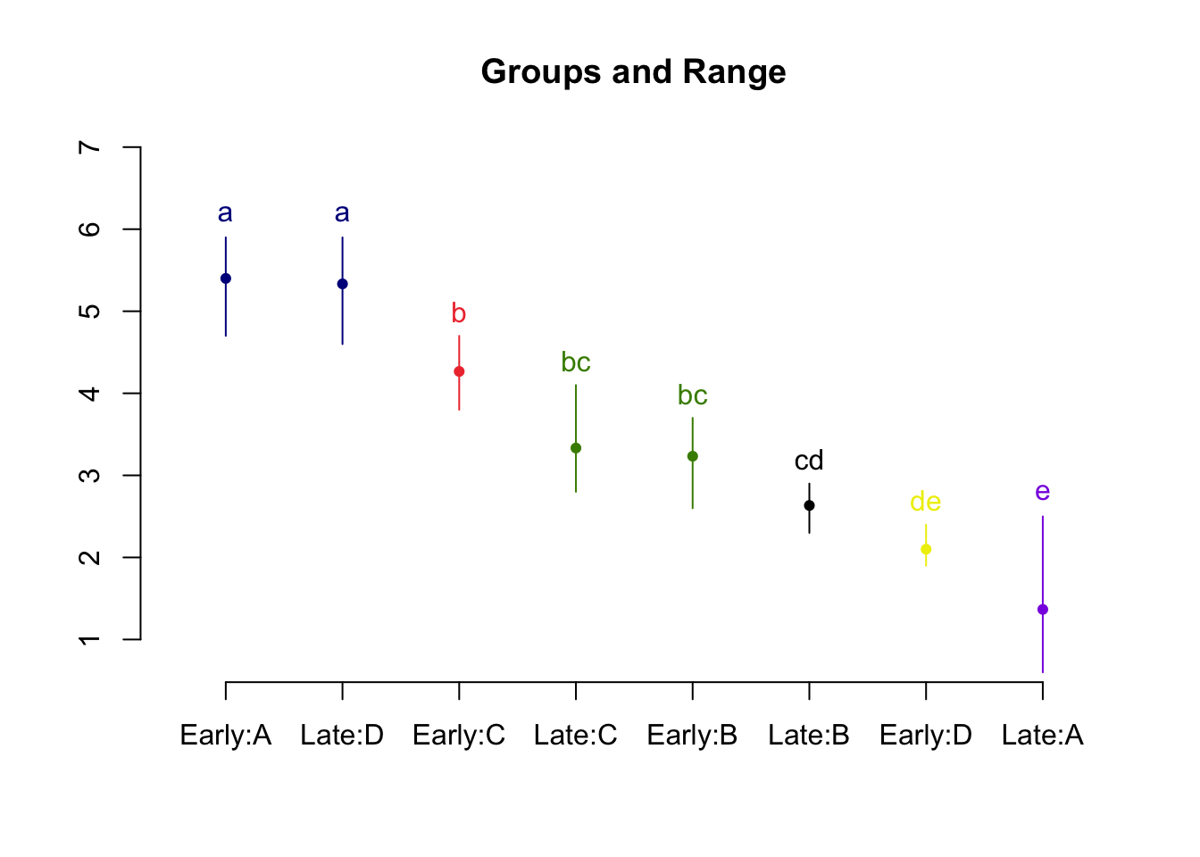
# Do an interaction plot to help interpret the results:
attach(weeds)
interaction.plot(chemical, time, drymatter, type = "l",
                 col = c("blue", "red"),
main = "Interaction Plot for Weed Control Example") 